Separately excited DC generators
(Refer Slide Time: 00:28)
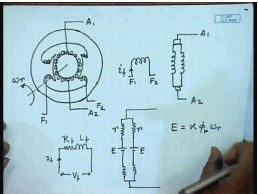
The cross section of a two pole DC Machine will look somewhat like this. These are the armature terminals, you also have field winding. These are the field terminals. schematically this is the shaft, can be represented as the field winding with the current i f and armature winding, it is to be noted that although you have a physical single field winding the armature winding represented in this schematic diagram does not really exist in the actual machine. In the actual machine as the armature rotates the constituent coils of these two parallel paths keeps changing, but overall the structure looks like this therefore, it is reasonable to represent the armature of a DC machine by a parallel connection of several coils. The individual constituent coils may change, but the number of coils between two brushes remains always constant number of parallel paths being equal to the number of poles for lab connected machine and equal to two for wave machine.
Now, if this armature is rotated at speed omega R then we have seen that each of this parallel path will have a induced voltage. And of course, the windings will also have their resistance, as well as inductance. Similarly the field winding will have its resistance and inductance, E as we have seen before is given by back E M F constant k flux per pole phi p into omega R, since these windings are identical the induced voltage are also identical.
(Refer Slide Time: 04:58)
Therefore these two parallel braches of our DC machine can be replaced by a single branch. This is the field winding, this is the armature winding. Let the armature voltage be v a this in plus this in minus and the motoring mode that the current, generating mode the current be i a, it is resistance is r a, this is E and this is the inductance L a for steady state operation the currents i a v a i a V f these are all DC. Therefore, the inductance do not play any role in determining the steady state behavior of a DC machine therefore, we can neglect the inductance for steady state operation.
Hence the field circuit can be represented by the simply the field resistance and the armature circuit by the armature resistance and the induced voltage E. Sometimes the contact resistance of the brushes are also modeled there are different ways of doing it. In can be modeled as a resistance, but more often not the drop across the brush is more or less constant. Therefore, it is reasonable to assume the total brush drop as another voltage of fixed magnitude, which is independent of all other machines parameters or variables like armature current or rotational speed this is called the brush contact drop, normally is above two volts and this is the terminal voltage V t.
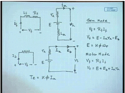
Therefore the steady state equation of a DC machine can be written as V f equal to R f I f, V t equal to E minus I a r a minus E brush, many a times this brush contact drop is neglected and E equal to k phi omega r, where omega r is the rotational speed of the armature. Now, this equation has been written with generator convention in mind that is assuming that the DC machine works as a generator. So, this is generator mode of operation for motor mode the direction of armature current will reverse. So, you will write V f equal to R f I f, V t equal to E plus E b plus I a r a.
The generated torque is always given by k phi I a, in the motoring mode the torque assists the motion that is, it rotates the machine in the generating mode it opposes motion. So, these are the basic equations steady state equations of a DC machine and depending on whether it is operating as a motor or generator, we will take the appropriate set of equations. Now, we can see that, these are simple linear algebraic equation except the relationship between I f and phi f.
(Refer Slide Time: 11:06)
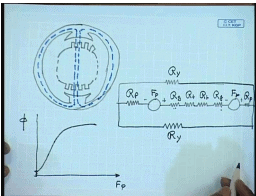
This relationship is not normally linear, because of magnetic saturation of the DC machine. The DC machine magnetic circuit can be drawn in a simplified way as given below. This is the armature which has slots and teethes on them, this is the pole. The flux path through the machine can be streps like this, the main flux path. So, the magnetic circuit of a DC machine can be drawn this manner. This is the m m f source due to the field coil on one pole, this is the m m f source on the second pole, this is the reluctance of the first air gap, this is the reluctance of the second air gap, these are the reluctance of the armature teeth, this is the reluctance of the pole body and these are the reluctance of the stator core. As we see from this magnetic equivalent circuit that, in this except for the reluctance of the air gap, now all other flux path contains iron which is a ferromagnetic material and shows prominent saturation.
Therefore as the field m m f F p increases the field flux phi initially rises in a linear manner as long as the iron remains unsaturated, but later on it shows a predominant saturation characteristics and becomes flat. Not only that the iron body also shows a residual magnetism, which is present in the iron if even when there is no field excitation this characteristic is important for the operation of a DC generator. So, it is excepted that the induced voltage in a DC generator will also follow similar pattern.
(Refer Slide Time: 16:23)
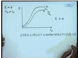
It is indeed so but it is customary to find out, since E is proportional to phi for a given and phi p, F p is proportional to I f. It is expected that if the induced voltage of a DC machine is plotted with respect to the field current. It will be similar to the characteristics of phi verses F p and operated at constant speed, these characteristics can be experimentally determined for every DC machine and is called the open circuit characteristics or O C C In short. This is a important characteristics for every DC machine and can be obtained experimentally by exciting the field winding from a separate source and keeping the armature terminals open and operating the machine as a generator at constant speed. and if the induced voltage is plotted verses field current at constant speed we obtain the O C C.
If the O C C is obtained at any given speed, let us say for a speed of N 1 the O C C for a different speed N 2 can be obtained from the O C C at N 1 by simply multiplying by proportionality constant. This O C C is obtained at speed N 2 is obtained by multiplying the O C C, the ordinate of the O C C by a factor N 1 by N 2. This is due to the fact that the back e m f, E induced voltage is proportional to N. It is to be emphasized that during the determination of O C C the field winding is excited separately and the armature terminals are kept open the machine is also operated as a generator at constant speed. A few other things, while determining the O C C the field current should be either continuously increased or decreased. It should not be, it should not alternate, because if it alternates then the flux in the core will show a local hysteresis and will introduce error in the O C C.
(Refer Slide Time: 20:08)
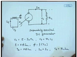
We have seen in our pervious class, that the field winding of a DC machine can be connected in many different ways. This is the armature terminal, this is the armature terminal this is the field terminal, when a field winding is excited from a separate DC source produce a flux phi, this is called a separately excited DC machine. For this separately excited DC generator, we can write the terminal voltage V t equal to induced voltage E minus I a r a and applied field voltage V f equal to R f I f, E equal to k phi I a and phi is some non-linear function of I F. The torque generated T e developed torque equal to k phi I a.
Since the armature terminals supplies the load. So, armature current is same as the load current I L. It is to be noted that this generator can either supply a standalone restive load R L in which case we have the further relation V t equal to R L I a or it can be connected to a DC bus having a terminal voltage equal to V t.
(Refer Slide Time: 23:15)
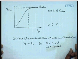
The O C C for separately excited machine generator can be obtained by running the generator at a constant speed and then increasing the field excitation slowly. So, that the terminal voltage when the armature terminals are open reaches a value which is larger than the rated value of the, if this is the rated value rated terminal voltage. Then the O C C is determined up to a value which is about 125 percent of V rated, this O C C is normally obtained at the rated speed of the generator.
However as we have mentioned earlier O C C for any other speed can be obtained by multiplying the O C C of the generator at rated speed by the ratio of the speed. However, it is more important for at least a generator to find out, what is called it is output characteristics or the external characteristics? This one is the open circuit characteristic or O C C. For a DC generator supplying a load as shown here, it will be more important to find out its external characteristics or the output characteristics. This is a plot of the terminal voltage V t verses the load current I L, which is same as I a in this case for constant speed N equal to N rated and I F equal to I F rated, where I F rated is the field current required to produce rated voltage at no load.
(Refer Slide Time: 26:44)
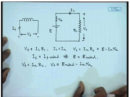
So, under load condition, this is the equivalent circuit of the DC generator. From this we can easily say V t equal to I L R L, I L equal to I a hence, V t equal to I a R L this is also equal to E minus I a r a. Now, these set of equations can be if I F equal to constant would imply, if the machine is operated at constant speed E equal to constant at E rated. So, the operating point can be found out from this relation V t equal to I a R L and V t by the intersection of these two straight lines E rated minus I a r a.
(Refer Slide Time: 29:13)
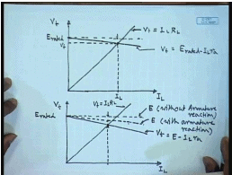
This is, if it is E rated and this is I L, one would expect that as the machine is loaded the terminal voltage will fall linearly. For a given load resistance, the terminal voltage also obeys the first equation, the load line equation. So, this equation represents V t equal to E rated minus I L r a, while the load line equation is given by V t equal to I L R L. So, for a given resistance L the operating point is given by the intersection of these two characteristics. This is the operating V t and this is the I L and this is the drop due to armature resistance. The characteristics of V t verses I L is called the output characteristics or the external characteristics of the generator.
However this simple model neglects the effect of armature reaction, we have seen before that due to current flowing in the armature, the field flux is distorted the field flux at one half of the pole tip increases and in the other half it decreases. Now, if the machine is operating near the saturation zone, near the saturation point that decrease of the field flux due to armature reaction is more than the increase in the second other half of the pole due to increase in a peak. Therefore, there is a net reduction in flux per pole and hence due to armature reaction in a practical machine the value of induced voltage does not remain constant with increase in armature current. In fact, the armature voltage the induced voltage tends to drop.
So, without armature reaction with a constant field flux, the induced voltage would have remain constant at a value of E rated, but due to armature reaction there will be some drop. This is the induced voltage E without armature reaction and this is the induced voltage E with armature reaction. On top of this there will be a drop due to armature resistance therefore, this is at any, this is V t equal to E minus I L r a and this is the load line V t equal to I L R L the intersection point is here, there are two drops as we can see the first one is due to armature reaction and the second one is due to the armature resistance. Now, the drop due to armature resistance can be due to armature reaction, can be found out experimentally by operating the machine at constant speed and by gradually loading the machine with change in the field excitation current.
(Refer Slide Time: 36:19)
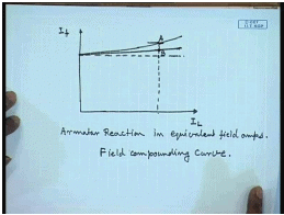
So, that so as to keep the terminal voltage constant at any desired value for any load current so this is a plot of I L verses I f. If there was no armature reaction then in order to keep the terminal voltage constant at any load current. You have to compensate only for the armature resistance drop and the characteristics would have been a straight line, but due to armature reaction some more increase in the field current will be required to overcome the drop due to armature reaction.
So, at any given load current one can find out the field ampere turns or field current required to compensate for the armature reaction drop from by calculating this magnitude A B. So, this way the armature drop in the armature voltage due to armature reaction can be expressed in terms of equivalent field current. Armature reaction in equivalent field amperes, this curve is called the field compounding curve. A field compounding curve is a plot of the field current verses the load current at constant rotational speed and at constant terminal voltage. That is it plots the field current required to keep the terminal voltage constant for any given load current when the machine operates at constant speed. It is important to understand that, the amount degree of saturation at the due to armature reaction is somewhat dependent on the terminal voltage of the DC generator.
Hence if the purpose is to find out the armature reaction m m f in equivalent field amperes, it is necessary to find out the field compounding curve at the desired terminal voltage. It is easy to understand that, this field compounding curve can be obtained at different speed and at different terminal voltage; however, in order to find out the equivalent field amperes for the armature reaction it is necessary to find out the field compounding curve at the required terminal voltage.
(Refer Slide Time: 40:20)
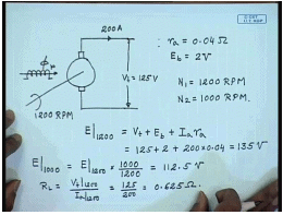
So, let us see, solve few problems to understand what has been discussed so far. Suppose we have a DC machine, separately excited DC machine, this machine as a armature resistance r a of 0.04 ohm, total brush contact drop E b equal to 2 volts. It supplies a load current of 200 ampere at a terminal voltage V t equal to 125 volts, when it is rotated at 1200 R P M. Question is if the rotational speed is reduced from 1200 R P M to N 2 equal to 1000 R P M, what will be the new armature current?
For this, let us first find out the induced voltage E at 1200 R P M neglecting, armature reaction E at 1200 R P M then will be terminal voltage plus brush contact drop plus armature resistance drop. Since back E M F is proportional to rotational speed E at 1000 R P M will be equal to E at 1200 R P M multiplied by 1000 divided by 1200 this comes to 112.5 volts. What is the load resistance R L? R L equal to V t at 1200 R P M divided by I a at 1200 R P M this is 125 by 200 equal to 0.625 ohm.
(Refer Slide Time: 45:05)
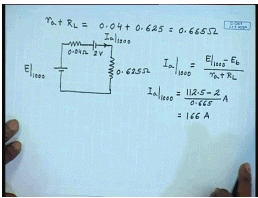
Hence, the total armature circuit resistance r a plus R L equal to 0.04 plus 625 equal to 0.665 ohm. At 1000 R P M therefore, you can draw the equivalent circuit as E at 1000 r a 0.04 ohm then E b equal to 2 volts then R L 0.625 ohm therefore, the current I a at 1000 R P M equal to E at 1000 R P M minus E b divided by r a plus R L or I a at 1000 R P M will be equal to 112.5 minus 2 divided by 0.665 ampere this comes to 166 ampere; however, in this problem we have neglected the armature reaction.
(Refer Slide Time: 47:40)
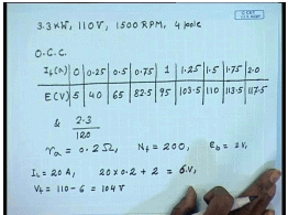
Let us try to solve a problem incorporating armature reaction, for this let us say we have a DC machine which is rated power is 3.3 kilowatt and rated terminal voltage is 110 volts, rated rotational speed is 1500 R P M, 4 pole. The O C C of this generator is given by the following data, no field current the residual voltage is 5 volts, 0.25 ampere this 40 volts, 0.5 ampere 65 volts, 0.75 ampere 82.5 volts, 1 ampere 95 volts, 1.25 amperes and at 2.3 ampere the voltage is 120 volts. The armature circuit resistance is r a equal to 0.2 ohm, number of field turns N f equal to 200, E b equal to 2 volts.
You can assume that the armature demagnetizing ampere turns is proportional to the armature current that is this line is a straight line and the effective demagnetizing ampere turns is equal to 1.5 times the armature current. So, you have to find out the terminal voltage of the machine at a given load current, when the machine is operated at constant speed. If we neglect armature reaction then let us say some load current I L equal to 20 amperes, the total armature circuit drop would have been 20 into 0.2 plus brush contact drop 2 volts equal to 6 volts and if the field excitation field current is at just as. So, that at no load the terminal voltage is 110 volt then at 20 ampere I L. V t would have been 110 minus 6 equal to 104 volts, but when you take armature reaction into account then the voltage becomes different.
(Refer Slide Time: 53:05)
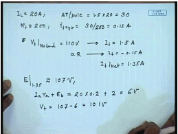
Let us again say a load current of 20 amperes, it is mentioned that ampere turns demagnetizing ampere turns per pole is 1.5 times the armature current. So, demagnetizing ampere turns equal to 30. Number of field turns is N F equal to 200 therefore, equivalent field amperes for the demagnetizing armature reaction ampere turns is 30 by 200 equal to 0.15 amperes. Now, in order to adjust V t at no load equal to 110 volts we see from this table the corresponding field current should have been this corresponds to a field current of I f equal to 1.5 amperes. The demagnetizing the armature reaction is equivalent to a demagnetizing field current a R armature reaction is I f equal to minus 0.15 ampere.
So, the effective I f net equal to 1.35 amperes, so the induced voltage with 1.35 ampere of field current will give you E at I f equal to 1.35 this approximately from that data it is approximately 107 volts. And the armature circuit drop is I a r a plus E b that is equal to 20 into 0.2 plus 2 equal to 6 volts therefore, the terminal voltage V t will be equal to 107 minus 6 equal to 101 volts. Therefore, we see without armature reaction, without considering armature reaction we are getting a terminal voltage of 104, but when armature reaction is included, the terminal voltage for the same field load current drops to 101 volt. This is the effect of armature reaction.
Thank you.


