Lecture 3 - Introduction to Digital Control - Electrical Engineering (EE) PDF Download

Lecture 3 - Introduction to Digital Control, Control Systems
1 Mathematical Modeling of Sampling Process
Sampling operation in sampled data and digital control system is used to model either the sample and hold operation or the fact that the signal is digitally coded. If the sampler is used to represent S/H (Sample and Hold) and A/D (Analog to Digital) operations, it may involve delays, finite sampling duration and quantization errors. On the other hand if the sampler is used to represent digitally coded data the model will be much simpler.
Following are two popular sampling operations:
1. Single rate or periodic sampling
2. Multi-rate sampling We would limit our discussions to periodic sampling only.
1.1 Finite pulse width sampler
In general, a sampler is the one which converts a continuous time signal into a pulse modulated or discrete signal. The most common type of modulation in the sampling and hold operation is the pulse amplitude modulation.
The symbolic representation, block digram and operation of a sampler are shown in Figure 1.
The pulse duration is p second and sampling period is T second. Uniform rate sampler is a linear device which satisfies the principle of superposition. As in Figure 1, p(t) is a unit pulse train with period T .
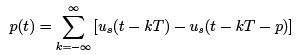
where us(t) represents unit step function. Assume that leading edge of the pulse at t = 0 coincides with t = 0. Thus fp∗(t) can be written as
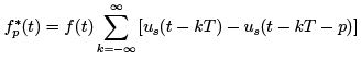

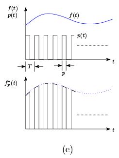
Figure 1: Finite pulse width sampler:(a)Symbolic representation (b)Block diagram (c)Operation
Frequency domain characteristics:
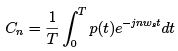
Since p(t) is a periodic function, it can be represented by a Fourier series, as
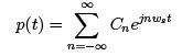
where
 is the sampling frequency and Cn’s are the complex Fourier series coefficients.
Since p(t) = 1 for 0 ≤ t ≤ p and 0 for rest of the period,
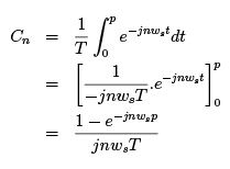
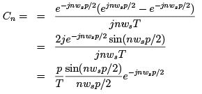
Cn can be rearranged as,
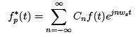
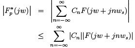
Since fp∗ (t) is also periodic, it can be written as
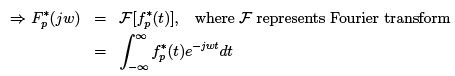
Using complex shifting theorem of Fourier transform
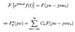
Since n is from −∞ to ∞, the above equation can also be written as
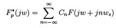
where,
The above equation implies that the frequency contents of the original signal f (t) are still present in the sampler output except that the amplitude is multiplied by the factor P/T.
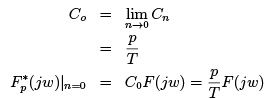
For n = 0, Cn is a complex quantity, the magnitude of which is,
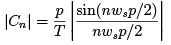
Magnitude of Fp∗(j w)
Sampling operation retains the fundamental frequency but in addition, sampler output also contains the harmonic components.
F (j w + j nws) for n = �1, �2, .....
According to Shannon’s sampling theorem, “if a signal contains no frequency higher than wc rad/sec, it is completely characterized by the values of the signal measured at instants of time separated by T = π/wc sec.”
Sampling frequency rate should be greater than the Nyquist rate which is twice the highest frequency component of the original signal to avoid aliasing.
If the sampling rate is less than twice the input frequency, the output frequency will be different from the input which is known as aliasing. The output frequency in that case is called alias frequency and the period is referred to as alias period.
The overlapping of the high frequency components with the fundamental component in the frequency spectrum is sometimes referred to as folding and the frequency is often known as folding frequency. The frequency wc is called Nyquist frequency.
A low sampling rate normally has an adverse effect on the closed loop stability. Thus, often we might have to select a sampling rate much higher than the theoretical minimum.
1.2 Flat-top approximation of finite-pulsewidth sampling
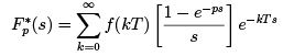
The Laplace transform of fp∗(t) can be written as
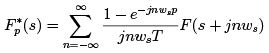
If the sampling duration p is much smaller than the sampling period T and the smallest time constant of the signal f (t), the sampler output can be approximated by a sequence of rectangular pulses since the variation of f (t) in the sampling duration will be less significant. Thus for k = 0, 1, 2, .........., fp∗ (t) can be expressed as an infinite series
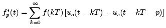
Taking Laplace transform,
Since p is very small, e−ps can be approximated by taking only the first 2 terms, as
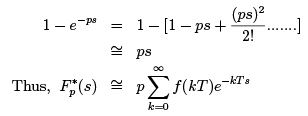
In time domain,
where, δ(t) represents the unit impulse function. Thus the finite pulse width sampler can be viewed as an impulse modulator or an ideal sampler connected in series with an attenuator with attenuation p.
1.3 The ideal sampler
In case of an ideal sampler, the carrier signal is replaced by a train of unit impulse as shown in Figure 2. The sampling duration p approaches 0, i.e., its operation is instantaneous.
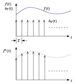
Figure 2: Ideal sampler operation
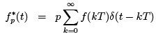
The output of an ideal sampler can be expressed as
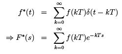
One should remember that practically the output of a sampler is always followed by a hold device which is the reason behind the name sample and hold device. Now, the output of a hold device will be the same regardless the nature of the sampler and the attenuation factor p can be dropped in that case. Thus the sampling process can be be always approximated by an ideal sampler or impulse modulator.
FAQs on Lecture 3 - Introduction to Digital Control - Electrical Engineering (EE)
| 1. What is digital control? |  |
| 2. What are the advantages of digital control over analog control? | |
| 3. How does digital control work? | |
| 4. What are the common applications of digital control? | |
| 5. What are the challenges in implementing digital control systems? | |


Top Courses for Electrical Engineering (EE)

shortcuts and tricks
,study material
,Semester Notes
,Sample Paper
,Summary
,video lectures
,MCQs
,Important questions
,Free
,Viva Questions
,Lecture 3 - Introduction to Digital Control - Electrical Engineering (EE)
,ppt
,practice quizzes
,Objective type Questions
,Exam
,mock tests for examination
,Previous Year Questions with Solutions
,Lecture 3 - Introduction to Digital Control - Electrical Engineering (EE)
,Extra Questions
,Lecture 3 - Introduction to Digital Control - Electrical Engineering (EE)
,past year papers
;


Lecture 3 - Introduction to Digital Control Free PDF Download
Importance of Lecture 3 - Introduction to Digital Control
Lecture 3 - Introduction to Digital Control Notes
Lecture 3 - Introduction to Digital Control Electrical Engineering (EE) Questions
Study Lecture 3 - Introduction to Digital Control on the App
|
© EduRev
|
Education Revolution
|


|


