Lecture 5 - Modeling Discrete Time Systems by Pulse Transfer Function - Electrical Engineering (EE) PDF Download

Lecture 5 - Modeling discrete-time systems by pulse transfer function, Control Systems
1 Motivation for using Z-transform
In general, control system design methods can be classified as:
conventional or classical control techniques
modern control techniques
Classical methods use transform techniques and are based on transfer function models, whereas modern techniques are based on modeling of system by state variable methods.
Laplace transform is the basic tool of the classical methods in continuous domain. In principle, it can also be used for modeling digital control systems. However typical Laplace transform expressions of systems with digital or sampled signals contain exponential terms in the form of eTs which makes the manipulation in the Laplace domain difficult. This can be regarded as a motivation of using Z-transform.
Let the output of an ideal sampler be denoted by f ∗(t).
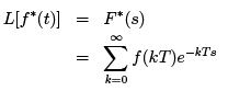
Since F ∗(s) contains the term e−kTs, it is not a rational function of s. When terms with e−Ts appear in a transfer function other than a multiplying factor, difficulties arise while taking the inverse Laplace. It is desirable to transfer the irrational function F ∗(s) to a rational function for which one obvious choice is:
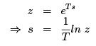
If, s = σ + j w,
Re z = eT σ cos wT
I m z = eT σ sin wT
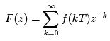
Z-transform:
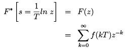
F (z ) is the Z-transform of f (t) at the sampling instants k.
In general, we can say that if f (t) is Laplace transformable then it also has a Z-transform.

2 Revisiting Z-Transforms
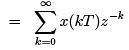
Z-transform is a powerful operation method to deal with discrete time systems. In considering Z-transform of a time function x(t), we consider only the sampled values of x(t), i.e., x(0), x(T ), x(2T )....... where T is the sampling period.
X (z) = Z [x(t)] = Z [x(kT )]
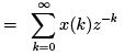
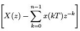
For a sequence of numbers x(k)
X (z) = Z [x(k)]
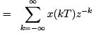
The above transforms are referred to as one sided z-transform. In one sided z-transform, we assume that x(t) = 0 for t < 0 or x(k) = 0 for k < 0. In two sided z-transform, we assume that −∞ < t < ∞ or k =, ±1, ±2, ±3, ........
X (z) = Z [x(kT )]
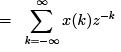
or for x(k)
X (z) = Z [x(k)]
The one sided z-transform has a convenient closed form solution in its region of convergence (ROC) for most engineering applications. Whenever X (z), an infinite series in z−1, converges outside the circle |z | = R, where R is the radius of absolute convergence, it is not needed each time to specify the values of z over which X (z ) is convergent.
|z| > R ⇒ convergent
|z| < R ⇒ divergent.
In one sided z-transform theory, while sampling a discontinuous function x(t), we assume that the function is continuous from the right, i.e., if discontinuity occurs at 0 we assume that x(0) = x(0+).
2.1 Z-Transforms of some elementary functions
Unit step function is defined as:
us(t) = 1, for t ≥ 0
= 0, for t < 0
Assuming that the function is continuous from right
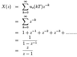
The above series converges if |z | > 1.
One should note that the Unit step sequence is defined as
us(k) = 1, for k = 0, 1, 2 · · ·
= 0, for k < 0
with a same Z-transform.
Unit ramp function is defined as:
ur (t) = t, for t ≥ 0
= 0, for t < 0
The Z-transform is:
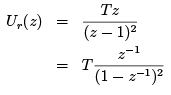
with ROC |z| > 1.
For a polynomial function x(k) = ak , the Z-transform is:
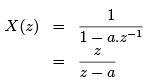
where ROC is |z| > a.
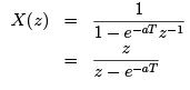
Exponential function is defined as:
x(t) = e−at, for t ≥ 0
= 0, for t < 0
We have x(kT ) = e−akT for k = 0, 1, 2 · · · . Thus,
Similarly Z-transforms can be computed for sinusoidal and other compound functions. One should refer the Z-transform table provided in the appendix.
2.2 Properties of Z- transform
1. Multiplication by a constant: Z [ax(t)] = aX (z), where X (z) = Z [x(t)].
2. Linearity: If x(k) = αf (k) ± β g(k), then X (z) = αF (z) ± β G(z).
3. Multiplication by ak : Z [ak x(k)] = X (a−1z)
4. Real shifting: Z [x(t − nT )] = z−nX (z) and z[x(t + nT )] = zn
5. Complex shifting: Z [e±atx(t)] = X (ze∓aT )
6. Initial value theorem: 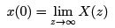
7. Final value theorem: 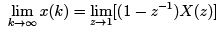
2.3 Inverse Z-transforms
Single sided Laplace transform and its inverse make a unique pair,i.e. if F (s) is the Laplace transform of f (t), then f (t) is the inverse Laplace transform of F (s). But the same is not true for Z-transform. Say f (t) is the continuous time function whose Z-transform is F (z ) then the inverse transform is not necessarily equal to f (t), rather it is equal to f (kT ) which is equal to f (t) only at the sampling instants. Once f (t) is sampled by an the ideal sampler, the information between the sampling instants is totally lost and we cannot recover actual f (t) from F (z ),
⇒ f (kT ) = Z −1[F (z)]
The transform can be obtained by using
→ Partial fraction expansion
→ Power series
→ Inverse formula.
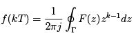
Inverse Z-transform formula:
2.4 Other Z-transform properties
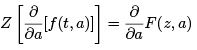
Partial differentiation theorem:
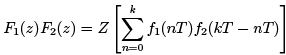
Real convolution theorem:
If f1(t) and f2(t) have z-transforms F1(z ) and F2(z ) and f1(t) = 0 = f2(t) for t < 0, then
Complex convolution:
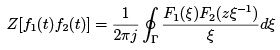
Γ : circle / closed path in z-plane which lie in the region 
σ1: radius of convergence ofF1(ξ )
σ1: radius of convergence of F2(ξ )
2.5 Limitation of Z-transform method
1. Ideal sampler assumption ⇒ z-transform represents the function only at sampling instants.
2. Non uniqueness of z-transform.
3. Accuracy depends on the magnitude of the sampling frequency ws relative to the highest frequency component contained in the function f (t).
4. A good approximation of f (t) can only be interpolated from f (kT ), the inverse z-transform of F (z) by connecting f (kT ) with a smooth curve.
2.6 Application of Z-transform in solving Difference Equation
One of the most important applications of Z-transform is in the solution of linear difference equations. Let us consider that a discrete time system is described by the following difference equation.
y(k + 2) + 0.5y(k + 1) + 0.06y(k) = −(0.5)k+1 with the initial conditions y(0) = 0, y(1) = 0. We have to find the solution y(k) for k > 0.
Taking z-transform on both sides of the above equation:
z2Y (z) + 0.5zY (z) + 0.06Y (z) = 
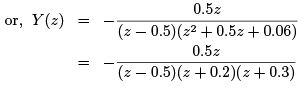
Using partial fraction expansion:
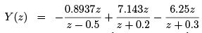
Taking Inverse Laplace: y(k) = −0.893(0.5)k + 7.143(−0.2)k − 6.25(−0.3)k
To emphasize the fact that y(k) = 0 for k < 0, it is a common practice to write the solution as: y(k) = −0.893(0.5)k us(k) + 7.143(−0.2)k us(k) − 6.25(−0.3)k us(k)
where us(k) is the unit step sequence.
FAQs on Lecture 5 - Modeling Discrete Time Systems by Pulse Transfer Function - Electrical Engineering (EE)
| 1. What is a pulse transfer function? |  |
| 2. How is a pulse transfer function different from a transfer function? | |
| 3. How is a pulse transfer function derived? | |
| 4. What are the advantages of modeling discrete-time systems using a pulse transfer function? | |
| 5. Can a continuous-time system be represented using a pulse transfer function? | |


Top Courses for Electrical Engineering (EE)

Exam
,shortcuts and tricks
,Semester Notes
,ppt
,mock tests for examination
,Viva Questions
,MCQs
,study material
,past year papers
,Sample Paper
,Previous Year Questions with Solutions
,Extra Questions
,practice quizzes
,Important questions
,Summary
,Objective type Questions
,Lecture 5 - Modeling Discrete Time Systems by Pulse Transfer Function - Electrical Engineering (EE)
,video lectures
,Lecture 5 - Modeling Discrete Time Systems by Pulse Transfer Function - Electrical Engineering (EE)
,Lecture 5 - Modeling Discrete Time Systems by Pulse Transfer Function - Electrical Engineering (EE)
,Free
;


Lecture 5 - Modeling Discrete Time Systems by Pulse Transfer Function Free PDF Download
Importance of Lecture 5 - Modeling Discrete Time Systems by Pulse Transfer Function
Lecture 5 - Modeling Discrete Time Systems by Pulse Transfer Function Notes
Lecture 5 - Modeling Discrete Time Systems by Pulse Transfer Function Electrical Engineering (EE) Questions
Study Lecture 5 - Modeling Discrete Time Systems by Pulse Transfer Function on the App
|
© EduRev
|
Education Revolution
|


|


