Lecture 6 - Modeling Discrete Time Systems by Pulse Transfer Function - Electrical Engineering (EE) PDF Download

Lecture 6 - Modeling discrete-time systems by pulse transfer function, Control Systems
1 Relationship between s-plane and z-plane
In the analysis and design of continuous time control systems, the pole-zero configuration of the transfer function in s-plane is often referred. We know that:
- Left half of s-plane ⇒ Stable region.
- Right half of s-plane ⇒ Unstable region.
For relative stability again the left half is divided into regions where the control loop transfer function poles should preferably be located.
Similarly the poles and zeros of a transfer function in z-domain govern the performance characteristics of a digital system.
One of the properties of F ∗(s) is that it has an infinite number of poles, located periodically with intervals of ±mws with m = 0, 1, 2, ....., in the s-plane where ws is the sampling frequency in rad/sec.
If the primary strip is considered, the path, as shown in Figure 1, will be mapped into a unit circle in the z-plane, centered at the origin. The mapping is shown in Figure 2.
Since
e(s+jmws)T = eTsej2πm
= eTs
= z
where m is an integer, all the complementary strips will also map into the unit circle.
1.1 Mapping guidelines
1. All the points in the left half s-plane correspond to points inside the unit circle in z-plane.
2. All the points in the right half of the s-plane correspond to points outside the unit circle.
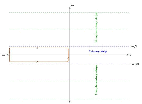
Figure 1: Primary and complementary strips in s-plane
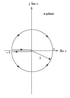
Figure 2: Mapping of primary strip in z-plane
3. Points on the j w axis in the s-plane correspond to points on the unit circle |z | = 1 in the
z-plane.
s = jw
z = eTs
= ejwT ⇒ magnitude = 1
1.2 Constant damping loci, constant frequency loci and constant damping ratio loci
Constant damping loci: The real part σ of a pole, s = σ + j w, of a transfer function in s-domain, determines the damping factor which represents the rate of rise or decay of time response of the system.
- Large σ represents small time constant and thus a faster decay or rise and vice versa.
- The loci in the left half s-plane (vertical line parallel to j w axis as in Figure 3(a)) denote positive damping since the system is stable
- The loci in the right half s-plane denote negative damping.
- Constant damping loci in the z-plane are concentric circles with the center at z = 0, as shown in Figure 3(b).
- Negative damping loci map to circles with radii > 1 and positive damping loci map to circles with radii < 1.
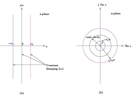
Figure 3: Constant damping loci in (a) s-plane and (b) z-plane
Constant frequency loci: These are horizontal lines in s-plane, parallel to the real axis as shown in Figure 4(a).

Figure 4: Constant frequency loci in (a) s-plane and (b) z-plane
Corresponding Z-transform:
z = eTs
= ejwT
When w = constant, it represents a straight line from the origin at an angle of θ = wT rad, measured from positive real axis as shown in Figure 4(b).
Constant damping ratio loci: If ξ denotes the damping ratio:
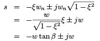
where wn is the natural undamped frequency and β = sin−1 ξ . If we take Z-transform
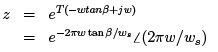
For a given ξ or β , the locus in s-plane is shown in Figure 5(a). In z-plane, the corresponding locus will be a logarithmic spiral as shown in Figure 5(b), except for ξ = 0 or β = 0o and ξ = 1 or β = 90o.
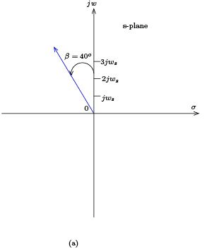
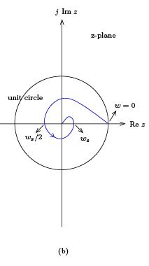
Figure 5: Constant damping ratio locus in (a) s-plane and (b) z-plane
FAQs on Lecture 6 - Modeling Discrete Time Systems by Pulse Transfer Function - Electrical Engineering (EE)
| 1. What is a pulse transfer function? |  |
| 2. How is a pulse transfer function different from a transfer function? | |
| 3. How can we model discrete time systems using a pulse transfer function? | |
| 4. What are the advantages of using a pulse transfer function in system modeling? | |
| 5. How can the pulse transfer function be used in control system design? | |


Top Courses for Electrical Engineering (EE)

Lecture 6 - Modeling Discrete Time Systems by Pulse Transfer Function - Electrical Engineering (EE)
,mock tests for examination
,Important questions
,Summary
,study material
,Sample Paper
,Objective type Questions
,ppt
,Exam
,Extra Questions
,past year papers
,Semester Notes
,practice quizzes
,MCQs
,Viva Questions
,Previous Year Questions with Solutions
,video lectures
,Lecture 6 - Modeling Discrete Time Systems by Pulse Transfer Function - Electrical Engineering (EE)
,Free
,shortcuts and tricks
,Lecture 6 - Modeling Discrete Time Systems by Pulse Transfer Function - Electrical Engineering (EE)
;


Lecture 6 - Modeling Discrete Time Systems by Pulse Transfer Function Free PDF Download
Importance of Lecture 6 - Modeling Discrete Time Systems by Pulse Transfer Function
Lecture 6 - Modeling Discrete Time Systems by Pulse Transfer Function Notes
Lecture 6 - Modeling Discrete Time Systems by Pulse Transfer Function Electrical Engineering (EE) Questions
Study Lecture 6 - Modeling Discrete Time Systems by Pulse Transfer Function on the App
|
© EduRev
|
Education Revolution
|


|


within 7 days!