Lecture 7 - Modeling Discrete Time Systems by Pulse Transfer Function - Electrical Engineering (EE) PDF Download

Lecture 7 - Modeling discrete-time systems by pulse transfer function, Control Systems
1 Pulse Transfer Function
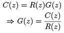
Transfer function of an LTI (Linear Time Invariant) continuous time system is defined as

where R(s) and C (s) are Laplace transforms of input r(t) and output c(t). We assume that initial condition are zero.
Pulse transfer function relates z-transform of the output at the sampling instants to the Ztransform of the sampled input. When the same system is sub ject to a sampled data or digital signal r∗(t), the corresponding block diagram is given in Figure 1.
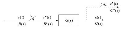
Figure 1: Block diagram of a system sub ject to a sampled input The output of the system is C (s) = G(s)R∗(s). The transfer function of the above system is difficult to manipulate because it contains a mixture of analog and digital components. Thus, it is desirable to express the system characteristics by a transfer function that relates r∗(t) to c ∗(t), a fictitious sampler output as shown in Figure 1. One can then write:
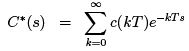
Since c(kT ) is periodic,
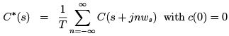
The detailed derivation of the above expression is omitted. Similarly,

Since R∗(s) is periodic R∗(s + j nWs) = R∗(s). Thus
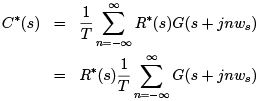
If we define G∗(s)  G(s + j nws), then C ∗(s) = R∗(s)G∗(s).

is known as pulse transfer function. Sometimes it is also referred to as the starred transfer function. If we now substitute z = eTs in the previous expression we will directly get the ztransfer function G(z) as
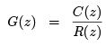
G(z) can also be defined as
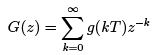
where g(kT ) denotes the sequence of the impulse response g(t) of the system of transfer function G(s). The sequence g(kT ), k = 0, 1, 2, .. is also known as impulse sequence.
Overall Conclusion
1. Pulse transfer function or z-transfer function characterizes the discrete data system responses only at sampling instants. The output information between the sampling instants is lost.
2. Since the input of discrete data system is described by output of the sampler, for all practical purposes the samplers can be simply ignored and the input can be regarded as r ∗(t).
Alternate way to arrive at G(z) = 
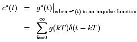
When the input is r∗(t),
c(t) = r(0)g(t) + r(T )g(t − T ) + ...
⇒ c(kT ) = r(0)g(kT ) + r(T )g((k − 1)T ) + ...
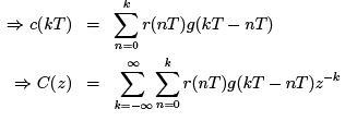
Using real convolution theorem
1.1 Pulse transfer of discrete data systems with cascaded elements
Care must be taken when the discrete data system has cascaded elements. Following two cases will be considered here.
- Cascaded elements are separated by a sampler
- Cascaded elements are not separated by a sampler
The block diagram for the first case is shown in Figure 2.
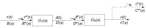
Figure 2: Discrete data system with cascaded elements, separated by a sampler
The input-output relations of the two systems G1 and G2 are described by
D(z) = G1(z)R(z)
and
C (z) = G2(z)D(z)
Thus the input-output relation of the overall system is
C (z) = G1(z)G2(z)R(z)
We can therefore conclude that the z-transfer function of two linear system separated by a sampler are the products of the individual z-transfer functions.
Figure 3 shows the block diagram for the second case. The continuous output C (s) can be
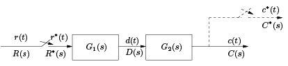
Figure 3: Discrete data system with cascaded elements, not separated by a sampler
written as
C (s) = G1(s)G2(s)R∗(s)
The output of the fictitious sampler is
C (z) = Z [G1(s)G2(s)] R(z) z-transform of the product G1(s)G2(s) is denoted as
Z [G1(s)G2(s)] = G1G2(z) = G2G1(z)
One should note that in general G1G2(z) = G1(z)G2(z), except for some special cases. The overall output is thus,
C (z) = G1G2(z)R(z)
1.2 Pulse transfer function of ZOH
As derived in lecture 4 of module 1, transfer function of zero order hold is
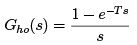
⇒ Pulse transfer function Gho(z)
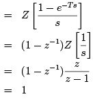
This result is expected because zero order hold simply holds the discrete signal for one sampling period, thus taking z-transform of ZOH would revert back its original sampled signal.
A common situation in discrete data system is that a sample and hold (S/H) device precedes a linear system with transfer function G(s) as shown in Figure 4. We are interested in finding the transform relation between r∗(t) and c∗(t).
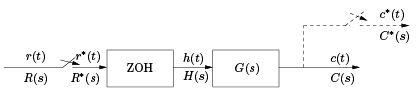
Figure 4: Block diagram of a system sub ject to a sample and hold process
z-transform of output c(t) is
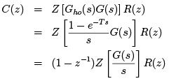
where  is the z-transfer function of an S/H device and a linear system.
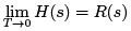
It was mentioned earlier that when sampling frequency reaches infinity a discrete data system may be regarded as a continuous data system. However, this does not mean that if the signal r(t) is sampled by an ideal sampler then r∗(t) can be reverted to r(t) by setting the sampling time T to zero. This simply bunches all the samples together. Rather, if the output of the sampled signal is passed through a hold device then setting the sampling time T to zero the original signal r(t) can be recovered. In relation with Figure 4,
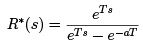
Example Consider that the input is r(t) = e−atus(t), where us(t) is the unit step function.
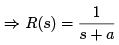
Laplace transform of sampled signal r∗(t) is
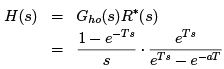
Laplace transform of the output after the ZOH is
When T → 0,
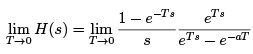
The limit can be calculated using L’ hospital’s rule. It says that:
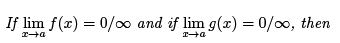
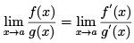
For the given example, x = T , f (T ) = 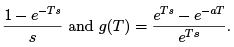 Both the expressions approach zero as T → 0. So,
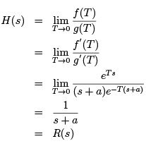
which implies that the original signal can be recovered from the output of the sample and hold device if the sampling period approaches zero.
FAQs on Lecture 7 - Modeling Discrete Time Systems by Pulse Transfer Function - Electrical Engineering (EE)
| 1. What is a pulse transfer function? |  |
| 2. How is a pulse transfer function different from a transfer function? | |
| 3. How can a pulse transfer function be derived? | |
| 4. What are the advantages of using a pulse transfer function? | |
| 5. Can a pulse transfer function be used to model continuous time systems? | |


Top Courses for Electrical Engineering (EE)

Semester Notes
,Summary
,Previous Year Questions with Solutions
,MCQs
,study material
,video lectures
,ppt
,Lecture 7 - Modeling Discrete Time Systems by Pulse Transfer Function - Electrical Engineering (EE)
,Free
,Exam
,shortcuts and tricks
,practice quizzes
,Important questions
,Objective type Questions
,Extra Questions
,Sample Paper
,Lecture 7 - Modeling Discrete Time Systems by Pulse Transfer Function - Electrical Engineering (EE)
,Viva Questions
,Lecture 7 - Modeling Discrete Time Systems by Pulse Transfer Function - Electrical Engineering (EE)
,past year papers
,mock tests for examination
;


Lecture 7 - Modeling Discrete Time Systems by Pulse Transfer Function Free PDF Download
Importance of Lecture 7 - Modeling Discrete Time Systems by Pulse Transfer Function
Lecture 7 - Modeling Discrete Time Systems by Pulse Transfer Function Notes
Lecture 7 - Modeling Discrete Time Systems by Pulse Transfer Function Electrical Engineering (EE) Questions
Study Lecture 7 - Modeling Discrete Time Systems by Pulse Transfer Function on the App
|
© EduRev
|
Education Revolution
|


|


