Lecture 9 - Modeling Discrete Time Systems by Pulse Transfer Function - Electrical Engineering (EE) PDF Download

Lecture 9 - Modeling discrete-time systems by pulse transfer function, Control Systems
1 Sampled Signal Flow Graph
It is known fact that the transfer functions of linear continuous time data systems can be determined from signal flow graphs using Mason’s gain formula.
Since most discrete data control systems contain both analog and digital signals, Mason’s gain formula cannot be applied to the original signal flow graph or block diagram of the system.
The first step in applying signal flow graph to discrete data systems is to express the system’s equation in terms of discrete data variables only.
Example 1: Let us consider the block diagram of a sampled data system as shown in Figure 1(a). We can write:
E(s) = R(s) − G(s)H (s)E∗(s) (1)
C(s) = G(s)E∗(s) (2)
The sampled data signal flow graph (SFG) is shown in Figure 1(b).
Taking pulse transform on both sides of equations (1) and (2), we get:
E∗(s) = R∗(s) − GH ∗(s)E ∗(s)
C∗(s) = G∗(s)E ∗(s)
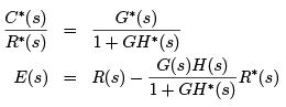
The above equations contain only discrete data variables for which the equivalent SFG will take a form as shown in Figure 1(c). If we apply Mason’s gain formula, we will get the following transfer functions.
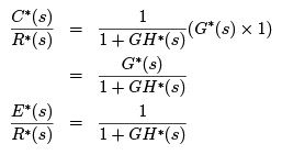
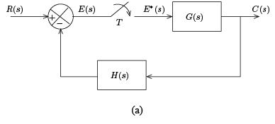
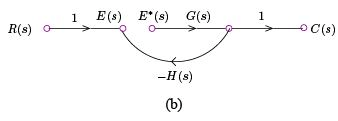
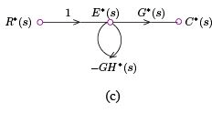
Figure 1: (a) Block diagram, (b) sampled signal flow graph and (c) equivalent signal flow graph for Example 1
The composite signal flow graph is formed by combining the equivalent and the original sampled signal flow graphs as shown in Figure 2.
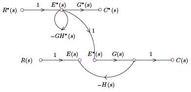
Figure 2: Composite signal flow graph for Example 1
The transfer function between the inputs and continuous data outputs are obtained from composite SFG using Mason’s gain formula.
In the composite SFG, the output nodes of the sampler on the sampled SFG are connected to the same nodes on equivalent SFG with unity gain. If we apply Mason’s gain formula to the composite SFG:
Example 2: Consider the block diagram as shown in Figure 3(a).
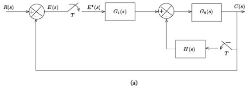
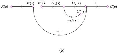
Figure 3: (a) Block diagram and (b) sampled signal flow graph for Example 2
The input output relations:
E(s) = R(s) − C (s) (3)
C(s) = (G1(s)E∗(s) − H (s)C∗(s))G2(s) (4)
= G1(s)G2(s)E∗(s) − G2(s)H (s)C∗(s) (5)
The sampled SFG is shown in Figure 3(b).
To find out the composite SFG, we take pulse transform on equations (5) and (3):
C∗(s) = G1G∗2(s)E ∗(s) − G2H ∗(s)C ∗(s)
E∗(s) = R∗(s) − C ∗(s)
= R∗(s) − G1G∗2(s)E ∗(s) + G2H ∗(s)C ∗(s)
The composite SFG is shown in Figure 4.
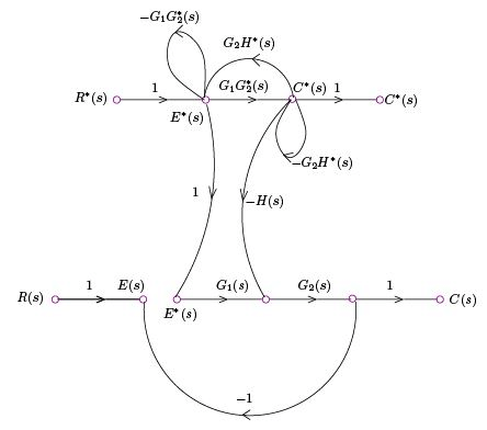
Figure 4: Composite signal flow graph for Example 2
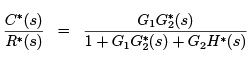
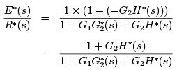
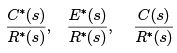 can be computed from Mason’s gain formula, as:
 .
.
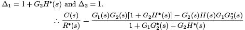
To derive  : Number of forward paths = 2 and the corresponding gains are
⇒ 1 × 1 × G1(s) × G2(s) = G1(s)G2(s)
⇒ 1 × G1G∗2(s) × (−H (s)) × G2(s) = −G2(s)H (s)G1G∗2(s)
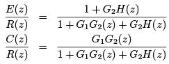
In Z-domain,
The sampled signal flow graph is not the only signal flow graph method available for discretedata systems. The direct signal flow graph is an alternate method which allows the evaluation of the input-output transfer function of discrete data systems by inspection. This method depends on an entirely different set of terminologies and definitions than those of Mason’s signal flow graph and will be omitted in this course.
Practice Problem 1.
Draw the composite signal flow graph of the system represented by the block diagram shown in Figure 5.
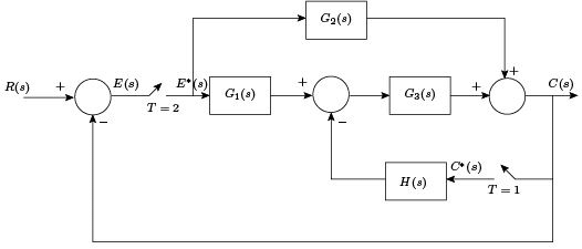
Figure 5: Block diagram for Exercise 1
Find out the closed loop discrete transfer function  if
if
 .
.
where Gh0(s) represents zero order hold.
FAQs on Lecture 9 - Modeling Discrete Time Systems by Pulse Transfer Function - Electrical Engineering (EE)
| 1. What is a pulse transfer function and how is it used to model discrete time systems? |  |
| 2. What are the advantages of modeling discrete time systems using pulse transfer function? | |
| 3. How can one determine the pulse transfer function of a discrete time system? | |
| 4. How is the pulse transfer function used in control system design? | |
| 5. What are some practical applications of modeling discrete time systems using pulse transfer function? | |


Top Courses for Electrical Engineering (EE)

Semester Notes
,Free
,Summary
,Viva Questions
,Objective type Questions
,Exam
,shortcuts and tricks
,Extra Questions
,video lectures
,Lecture 9 - Modeling Discrete Time Systems by Pulse Transfer Function - Electrical Engineering (EE)
,Previous Year Questions with Solutions
,practice quizzes
,Lecture 9 - Modeling Discrete Time Systems by Pulse Transfer Function - Electrical Engineering (EE)
,Sample Paper
,mock tests for examination
,past year papers
,Important questions
,Lecture 9 - Modeling Discrete Time Systems by Pulse Transfer Function - Electrical Engineering (EE)
,ppt
,study material
,MCQs
;


Lecture 9 - Modeling Discrete Time Systems by Pulse Transfer Function Free PDF Download
Importance of Lecture 9 - Modeling Discrete Time Systems by Pulse Transfer Function
Lecture 9 - Modeling Discrete Time Systems by Pulse Transfer Function Notes
Lecture 9 - Modeling Discrete Time Systems by Pulse Transfer Function Electrical Engineering (EE) Questions
Study Lecture 9 - Modeling Discrete Time Systems by Pulse Transfer Function on the App
|
© EduRev
|
Education Revolution
|


|


