Lecture 10 - Stability Analysis of Discrete Time Systems - Electrical Engineering (EE) PDF Download

Lecture 10 - Stability analysis of discrete time systems, Control Systems
1 Stability Analysis of closed loop system in z-plane
Stability is the most important issue in control system design. Before discussing the stability test let us first introduce the following notions of stability for a linear time invariant (LTI) system.
1. BIBO stability or zero state stbaility
2. Internal stability or zero input stability
Since we have not introduced the concept of state variables yet, as of now, we will limit our discussion to BIBO stability only.
An initially relaxed (all the initial conditions of the system are zero) LTI system is said to be BIBO stable if for every bounded input, the output is also bounded.
However, the stability of the following closed loop system
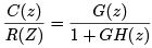
can be determined from the location of closed loop poles in z-plane which are the roots of the characteristic equation
1 + GH (z) = 0
1. For the system to be stable, the closed loop poles or the roots of the characteristic equation must lie within the unit circle in z-plane. Otherwise the system would be unstable.
2. If a simple pole lies at |z | = 1, the system becomes marginally stable. Similarly if a pair of complex conjugate poles lie on the |z | = 1 circle, the system is marginally stable. Multiple poles on unit circle make the system unstable.
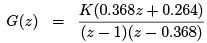
Example 1: Determine the closed loop stability of the system shown in Figure 1 when K = 1.
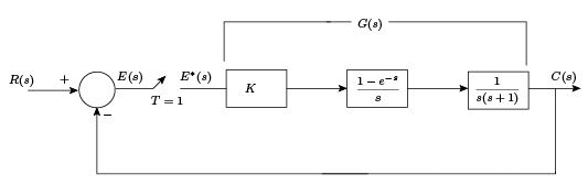
Figure 1: Example 1
Solution:
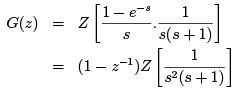
Since H (s) = 1,
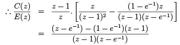
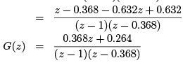
We know that the characteristics equation is ⇒ 1 + G(z) = 0
⇒ (z − 1)(z − 0.368) + 0.368z + 0.264 = 0
⇒ z2 − z + 0.632 = 0
⇒ z1 = 0.5 + 0.618j
⇒ z2 = 0.5 − 0.618j
Since |z1| = |z2| < 1, the system is stable.
Three stability tests can be applied directly to the characteristic equation without solving for the roots.
→ Schur-Cohn stability test
→ Jury Stability test
→ Routh stability coupled with bi-linear transformation.
Other stability tests like Lyapunov stability analysis are applicable for state space system models
which will be discussed later. Computation requirements in Jury test is simpler than SchurCohn when the co-efficients are real which is always true for physical systems.
1.1 Jury Stability Test
Assume that the characteristic equation is as follows,
P (z) = a0zn + a1zn−1 + ... + an−1z + an
where a0 > 0.
Jury Table
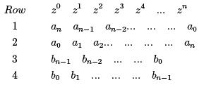
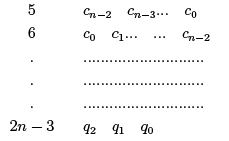
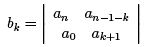
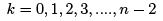
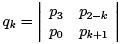
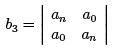
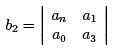
where,
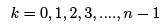
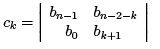
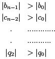
This system will be stable if:
1. |an| < a0
2. P (z )|z=1 > 0
3. P (z)|z=−1 > 0 for n even and P (z)|z=−1 < 0 for n odd
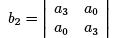
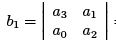
4.
Example 2: The characteristic equation: P (z) = z4 − 1.2z3 + 0.07z2 + 0.3z − 0.08 = 0
Thus, a0 = 1 a1 = −1.2 a2 = 0.07 a3 = 0.3 a4 = −0.08
We will now check the stability conditions.
1. |an| = |a4| = 0.08 < a0 = 1 ⇒ First condition is satisfied.
2. P (1) = 1 − 1.2 + 0.07 + 0.3 − 0.08 = 0.09 > 0 ⇒ Second condition is satisfied.
3. P (−1) = 1 + 1.2 + 0.07 − 0.3 − 0.08 = 1.89 > 0 ⇒ Third condition is satisfied.
Jury Table
 = 0.0064 − 1 = −0.9936
 = −0.08 × 0.3 + 1.2 = 1.176
Rest of the elements are also calculated in a similar fashion. The elements are b1 = −0.0756 b0 = −0.204 c2 = 0.946 c1 = −1.184 c0 = 0.315. One can see
|b3| = 0.9936 > |b0| = 0.204
|c2| = 0.946 > |c0| = 0.315
All criteria are satisfied. Thus the system is stable.
Example 3 The characteristic equation: P (z) = z3 − 1.3z2 − 0.08z + 0.24 = 0
Thus a0 = 1 a1 = −1.3 a2 = −0.08 a3 = 0.24.
Stability conditions are:
1. |a3| = 0.24 < a0 = 1 ⇒ First condition is satisfied.
2. P (1) = 1 − 1.3 − 0.08 + 0.24 = −0.14 < 0 ⇒ Second condition is not satisfied.
Since one of the criteria is violated, we may stop the test here and conclude that the system is unstable. P (1) = 0 or P (−1) = 0 indicates the presence of a root on the unit circle and in that case the system can at the most become marginally stable if rest of the conditions are satisfied.
The stability range of a parameter can also be found from Jury’s test which we will see in the next example.
Example 4: Consider the system shown in Figure 1. Find out the range of K for which the system is stable.
Solution:
The closed loop transfer function: 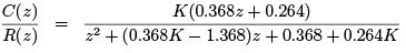
Characteristic equation: P (z) = z2 + (0.368K − 1.368)z + 0.368 + 0.264K = 0
Since it is a second order system only 3 stability conditions will be there.
1. |a2| < a0 2. P (1) > 0
3. P (−1) > 0 since n = 2=even. This implies: 1. |0.368 + 0.264K | < 1 ⇒ 2.39 > K > −5.18
2. P (1) = 1 + (0.368K − 1.368) + 0.368 + 0.264K = 0.632K > 0 ⇒ K > 0
3. P (−1) = 1 − (0.368K − 1.368) + 0.368 + 0.264K = 2.736 − 0.104K > 0 ⇒ 26.38 > K
Combining all, the range of K is found to be 0 < K < 2.39.
If K = 2.39, system becomes critically stable.
The characteristics equation becomes:
z2 − 0.49z + 1 = 0 ⇒ z = 0.244 ± j 0.97
Sampling period T = 1 sec.
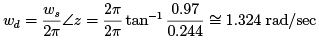
The above frequency is the frequency of sustained oscillation.
1.2 Singular Cases
When some or all of the elements of a row in the Jury table are zero, the tabulation ends prematurely. This situation is referred to as a singular case. It can be avoided by expanding or contracting unit circle infinitesimally by an amount ∈ which is equivalent to move the roots of P (z ) off the unit circle. The transformation is:
z1 = (1 + ∈)z
where ∈ is a very small number. When ∈ is positive the unit circle is expanded and when ∈ is negative the unit circle is contracted. The difference between the number of zeros found inside or outside the unit circle when the unit circle is expanded or contracted is the number of zeros on the unit circle. Since (1 + ∈)nz n ≌ (1 + n∈)z n for both positive and negative ∈, the transformation requires the coefficient of the zn term be multiplied by (1 + n∈).
Example 5: The characteristic equation: P (z) = z3 + 0.25z2 + z + 0.25 = 0
Thus, a0 = 1 a1 = 0.25 a2 = 1 a3 = 0.25.
We will now check the stability conditions.
1. |an| = |a3| = 0.25 < a0 = 1 ⇒ First condition is satisfied.
2. P (1) = 1 + 0.25 + 1 + 0.25 = 2.5 > 0 ⇒ Second condition is satisfied.
3. P (−1) = −1 + 0.25 − 1 + 0.25 = −1.5 < 0 ⇒ Third condition is satisfied.
Jury Table
 = 0.0625 − 1 = −0.9375
 = 0.25 − 0.25 = 0
Thus the tabulation ends here and we know that some of the roots lie on the unit circle. If we replace z by (1 + ∈)z , the characteristic equation would become:
(1 + 3∈)z3 + 0.25(1 + 2∈)z2 + (1 + ∈)z + 0.25 = 0
First three stability conditions are satisfied.
Jury Table
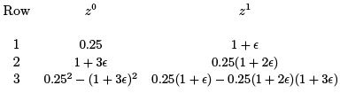

|b2| = |0.0625 − (1 + 6∈ + 9∈2)| and |b0| = |1 + 3.875∈ + 3∈2 − 0.0625|. Since, when ∈ → 0+, 1 + 6∈ + 9∈2 > 1 + 3.875∈ + 3∈2, thus |b2| > |b0| which implies that the roots which are not on the unit circle are actually inside it and the system is marginally stable.
FAQs on Lecture 10 - Stability Analysis of Discrete Time Systems - Electrical Engineering (EE)
| 1. What is stability analysis of discrete time systems? |  |
| 2. How is stability of discrete time systems determined? | |
| 3. What are the different types of stability in discrete time systems? | |
| 4. How does stability analysis impact the performance of discrete time systems? | |
| 5. What are some applications of stability analysis in discrete time systems? | |


Top Courses for Electrical Engineering (EE)

past year papers
,mock tests for examination
,shortcuts and tricks
,Sample Paper
,Summary
,Important questions
,Objective type Questions
,Exam
,MCQs
,study material
,Lecture 10 - Stability Analysis of Discrete Time Systems - Electrical Engineering (EE)
,Viva Questions
,Extra Questions
,Previous Year Questions with Solutions
,Lecture 10 - Stability Analysis of Discrete Time Systems - Electrical Engineering (EE)
,ppt
,Lecture 10 - Stability Analysis of Discrete Time Systems - Electrical Engineering (EE)
,practice quizzes
,video lectures
,Free
,Semester Notes
;


Lecture 10 - Stability Analysis of Discrete Time Systems Free PDF Download
Importance of Lecture 10 - Stability Analysis of Discrete Time Systems
Lecture 10 - Stability Analysis of Discrete Time Systems Notes
Lecture 10 - Stability Analysis of Discrete Time Systems Electrical Engineering (EE) Questions
Study Lecture 10 - Stability Analysis of Discrete Time Systems on the App
|
© EduRev
|
Education Revolution
|


|


within 7 days!