Lecture 11 - Stability Analysis of Discrete Time Systems - Electrical Engineering (EE) PDF Download

Lecture 11 - Stability analysis of discrete time systems, Control Systems
1 Stability Analysis using Bilinear Transformation and Routh Stability Criterion
Another frequently used method in stability analysis of discrete time system is the bilinear transformation coupled with Routh stability criterion. This requires transformation from z -plane to another plane called w-plane.
The bilinear transformation has the following form.
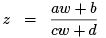
where a, b, c, d are real constants. If we consider a = b = c = 1 and d = −1, then the transformation takes a form

or, 
This transformation maps the inside of the unit circle in the z -plane into the left half of the w-plane. Let the real part of w be α and imaginary part be β ⇒ w = α + j β . The inside of the unit circle in z -plane can be represented by:
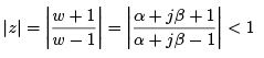

Thus inside of the unit circle in z -plane maps into the left half of w-plane and outside of the unit circle in z -plane maps into the right half of w-plane. Although w-plane seems to be similar to s-plane, quantitatively it is not same.
In the stability analysis using bilinear transformation, we first substitute  in the characteristics equation P (z ) = 0 and simplify it to get the characteristic equation in w-plane as Q(w) = 0. Once the characteristics equation is transformed as Q(w) = 0, Routh stability criterion is directly used in the same manner as in a continuous time system.
We will now solve the same examples which were used to understand the Jury’s test.
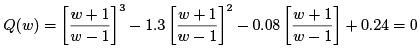
Example 1 The characteristic equation: P (z) = z3 − 1.3z2 − 0.08z + 0.24 = 0
Transforming P (z) into w-domain:
or, Q(w) = 0.14w3 − 1.06w2 − 5.1w − 1.98 = 0
We can now construct the Routh array as
w3 0.14 −5.1
w2 −1.06 −1.98
w1 −5.36
w0 −1.98
There is one sign change in the first column of the Routh array. Thus the system is unstable with one pole at right hand side of the w-plane or outside the unit circle of z -plane.
Example 2: The characteristic equation: P (z) = z4 − 1.2z3 + 0.07z2 + 0.3z − 0.08 = 0
Transforming P (z) into w-domain:

or, Q(w) = 0.09w4 + 1.32w3 + 5.38w2 + 7.32w + 1.89 = 0
We can now construct the Routh array as
w4 0.09 5.38 1.89
w3 1.32 7.32
w2 4.88 1.89
w1 6.81
w0 1.89
All elements in the first column of Routh array are positive. Thus the system is stable.
Example 3: Consider the system shown in Figure 1. Find out the range of K for which the system is stable.
Solution:
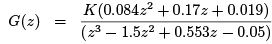
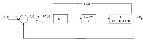
Figure 1: Figure for Example 3
Characteristic equation:
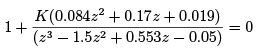
or, P (z) = z3 + (0.084K − 1.5)z2 + (0.17K + 0.553)z + (0.019K − 0.05) = 0
Transforming P (z) into w-domain:

or, Q(w) = (0.003 + 0.27K )w3 + (1.1 − 0.11K )w2 + (3.8 − 0.27K )w + (3.1 + 0.07K ) = 0
We can now construct the Routh array as
w3 0.003 + 0.27K 3.8 − 0.27K
w2 1.1 − 0.11K 3.1 + 0.07K
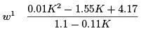
w0 3.1 + 0.07K
The system will be stable if all the elements in the first column have same sign. Thus the conditions for stability, in terms of K , are
0.003 + 0.27K > 0 ⇒ K > −0.011
1.1 − 0.11K > 0 ⇒ K < 10
0.01K 2 − 1.55K + 4.17 > 0 ⇒ K < 2.74 or, K > 140.98
3.1 + 0.07K > 0 ⇒ K > −44.3
Combining above four constraints, the stable range of K can be found as
−0.011 < K < 2.74
1.1 Singular Cases
In Routh array, tabulation may end in occurance with any of the following conditions.
- The first element in any row is zero.
- All the elements in a single row are zero.
The remedy of the first case is replacing zero by a small number ∈ and then proceeding with the tabulation. Stability can be checked for the limiting case. Second singular case indicates one or more of the following cases.
- Pairs of real roots with opposite signs.
- Pairs of imaginary roots.
- Pairs of complex conjugate roots which are equidistant from the origin.
When a row of all zeros occurs, an auxiliary equation A(w) = 0 is formed by using the coefficients of the row just above the row of all zeros. The roots of the auxiliary equation are also the roots of the characteristic equation. The tabulation is continued by replacing the row of zeros by the coefficients of  .
.
Looking at the correspondence between w-plane and z-plane, when an all zero row occurs, we can conclude that following two scenarios are likely to happen.
- Pairs of real roots in the z -plane that are inverse of each other.
- Pairs of roots on the unit circle simultaneously.
Example 4: Consider the characteristic equation
P (z) = z3 − 1.7z2 − z + 0.8 = 0
Transforming P (z) into w-domain:
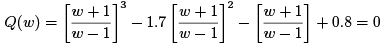
or, Q(w) = 0.9w3 + 0.1w2 − 8.1w − 0.9 = 0
The Routh array:
w3 0.9 −8.1
w2 0.1 −0.9
w1 0 0
The tabulation ends here. The auxiliary equation is formed by using the coefficients of w2 row, as:
A(w) = 0.1w2 − 0.9 = 0
Taking the derivative,
Thus the Routh tabulation is continued as
w3 0.9 −8.1
w2 0.1 −0.9
w1 0.2 0
w0 −0.9
As there is one sign change in the first row, one of the roots lie in w-plane is on the right hand side of the w-plane. This implies that one root in z -plane lies outside the unit circle.
To verify our conclusion, the roots of the polynomial z3 − 1.7z2 − z + 0.8 = 0, are found out to be z = 0.5, z = −0.8 and z = 2. Thus one can see that z = 2 lies outside the unit circle and it is inverse of z = 0.5 which caused the all zero row in w-plane.
FAQs on Lecture 11 - Stability Analysis of Discrete Time Systems - Electrical Engineering (EE)
| 1. What is stability analysis of discrete time systems? |  |
| 2. How is stability determined in discrete time systems? | |
| 3. Why is stability analysis important in engineering and control systems? | |
| 4. What are the different types of stability in discrete time systems? | |
| 5. How can one analyze the stability of a discrete time system using the root locus method? | |


Top Courses for Electrical Engineering (EE)

practice quizzes
,MCQs
,Summary
,Objective type Questions
,study material
,ppt
,Important questions
,past year papers
,Sample Paper
,Exam
,Extra Questions
,Semester Notes
,video lectures
,shortcuts and tricks
,mock tests for examination
,Viva Questions
,Previous Year Questions with Solutions
,Free
,Lecture 11 - Stability Analysis of Discrete Time Systems - Electrical Engineering (EE)
,Lecture 11 - Stability Analysis of Discrete Time Systems - Electrical Engineering (EE)
,Lecture 11 - Stability Analysis of Discrete Time Systems - Electrical Engineering (EE)
;


Lecture 11 - Stability Analysis of Discrete Time Systems Free PDF Download
Importance of Lecture 11 - Stability Analysis of Discrete Time Systems
Lecture 11 - Stability Analysis of Discrete Time Systems Notes
Lecture 11 - Stability Analysis of Discrete Time Systems Electrical Engineering (EE) Questions
Study Lecture 11 - Stability Analysis of Discrete Time Systems on the App
|
© EduRev
|
Education Revolution
|


|


