Lecture 13 - Time Response of Discrete Time Systems - Electrical Engineering (EE) PDF Download

Lecture 13 - Prototype second order system, Time Response of discrete time systems, Control Systems
1 Prototype second order system
The study of a second order system is important because many higher order system can be approximated by a second order model if the higher order poles are located so that their contributions to transient response are negligible. A standard second order continuous time system is shown in Figure 1. We can write
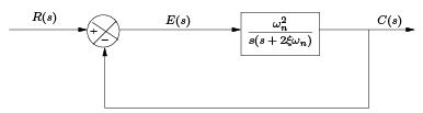
Figure 1: Block Diagram of a second order continuous time system
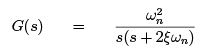
Closed loop: Gc(s)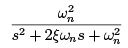
where, ξ = damping ratio
ωn = natural undamped frequency
Roots: 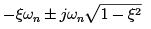
1.1 Comparison between continuous time and discrete time systems
The simplified block diagram of a space vehicle control system is shown in Figure 2. The ob jective is to control the attitude in one dimension, say in pitch. For simplicity vehicle body is considered as a rigid body.
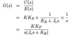
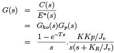
Position c(t) and velocity v(t) are fedback. The open loop transfer function can be calculated
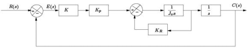
Figure 2: Space vehicle attitude control
as
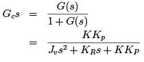
Closed loop transfer function is
KP = Position Sensor gain = 1.65 × 10⁶
KR = Rate sensor gain = 3.71 × 10⁵
K = Amplifier gain which is a variable
Jv = Moment of inertia = 41822
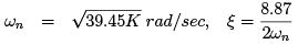
With the above parameters,
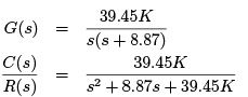
Characteristics equation ⇒ s2 + 8.87s + 39.45K = 0
Since the system is of 2nd order, the continuous time system will always be stable if KP , KR , K, Jv are all positive.
Now, consider that the continuous data system is sub ject to sampled data control as shown in Figure 3.
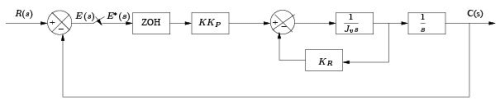
Figure 3: Discrete representation of space vehicle attitude control
For comparison purpose, we assume that the system parameters are same as that of the continuous data system.
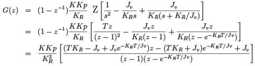
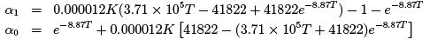
Characteristic equation of the closed loop system: z2 + α1z + α0 = 0, where
α1 = f1(K, Kp, KR, Jv)
α0 = f0(K, Kp, KR, Jv
Substituting the known parameters:
For stability
(1) |α0| < 1
(2) P (1) = 1 + α1 + α0 > 0 = 1 − e−8.87T > 0 always satisfied since T is positive
(3) P (−1) = 1 − α1 + α0 > 0
Choice of K and T : If we plot K versus T then according to conditions (1) and (3) the stable region is shown in Figure 4. Pink region represents the situation when condition (1) is satisfied but the (3) is not. Red region depicts the situation when condition (1) is satisfied, not the (3). Yellow is the stable region where both the conditions are satisfied. If we
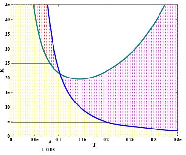
Figure 4: Kvs. T for space vehicle attitude control system want a comparatively large T , such as 0.2, the gain K is limited by the range K < 5. Similarly if we want a comparatively high gain such as 25, we have to go for T as small as 0.08 or even less.
From studies of continuous time systems it is well known that increasing the value of K generally reduces the damping ratio, increases peak overshoot, bandwidth and reduces the steady state error if it is finite and non zero.
2 Correlation between time response and root locations in s-plane and z-pane
The mapping between s-plane and z-plane was discussed earlier. For continuous time systems, the correlation between root location in s-plane and time response is well established and known.
- A root in negative real axis of s-plane produces an output exponentially decaying with time.
- Complex conjugate pole pairs in negative s-plane produce damped oscillations.
- Imaginary axis conjugate poles produce undamped oscillations
- Complex conjugate pole pairs in positive s-plane produce growing oscillations.
Digital control systems should be given special attention due to sampling operation. For example, if the sampling theorem is not satisfied, the folding effect can entirely change the true response of the system.
The pole-zero map and natural response of a continuous time second order system is shown in Figure 5.
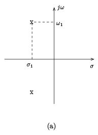
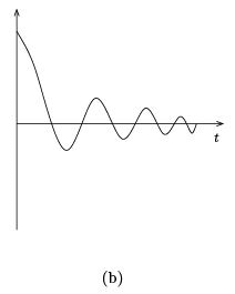
Figure 5: Pole zero map and natural response of a second order system
If the system is sub ject to sampling with frequency ωs < 2ω1, it will generate an infinite number of poles in the s-plane at s = σ1 ± jω1 + j nωs for n = ±1, ±2, ........ The sampling operation will fold the poles back into the primary strip where −ωs/2 < ω < ωs/2. The net effect is equivalent to having a system with poles at s = σ1 ± j (ωs − ω1). The corresponding plot is shown in Figure 6.
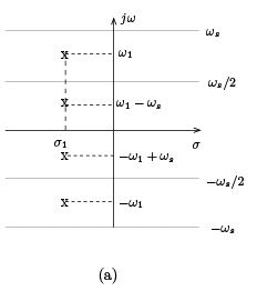
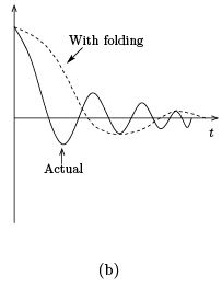
Figure 6: Pole zero map and natural response of a second order system Root locations in z-plane and the corresponding time responses are shown in Figure 7.
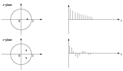
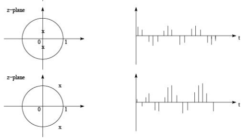
Figure 7: Pole zero map and natural response of a second order system
3 Dominant Closed Loop Pole Pairs
As in case of s-plane, some of the roots in z-plane have more effects on the system response than the others. It is important for design purpose to separate out those roots and give them the name dominant roots.
In s-plane, the roots that are closest to jω axis in the left plane are the dominant roots because the corresponding time response has slowest decay. Roots that are for away from jω axis correspond to fast decaying response.
- In Z-plane dominant roots are those which are inside and closest to the unit circle whereas insignificant region is near the origin.
- The negative real axis is generally avoided since the corresponding time response is oscillatory in nature with alternate signs.
Figure 8 shows the regions of dominant and insignificant roots in s-plane and z-plane.
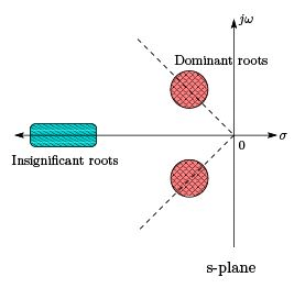

Figure 8: Pole zero map of a second order system
In s-plane the insignificant roots can be neglected provided the dc-gain (0 frequency gain) of the system is adjusted. For example,
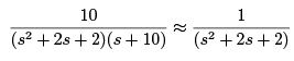
In z-plane, roots near the origin are less significant from the maximum overshoot and damping point of view.
However these roots cannot be completely discarded since the excess number of poles over zeros has a delay effect in the initial region of the time response, e.g., adding a pole at z = 0 would not effect the maximum overshoot or damping but the time response would have an additional delay of one sampling period.
The proper way of simplifying a higher order system in z-domain is to replace the poles near origin by Poles at z = 0 which will simplify the analysis since the Poles at z = 0 correspond to pure time delays.
FAQs on Lecture 13 - Time Response of Discrete Time Systems - Electrical Engineering (EE)
| 1. What is the time response of discrete time systems? |  |
| 2. How is the time response of discrete time systems different from continuous time systems? | |
| 3. What are some common examples of discrete time systems? | |
| 4. How can the time response of a discrete time system be analyzed? | |
| 5. What factors can influence the time response of discrete time systems? | |


Top Courses for Electrical Engineering (EE)

Lecture 13 - Time Response of Discrete Time Systems - Electrical Engineering (EE)
,ppt
,Viva Questions
,Previous Year Questions with Solutions
,mock tests for examination
,MCQs
,past year papers
,Objective type Questions
,shortcuts and tricks
,study material
,Lecture 13 - Time Response of Discrete Time Systems - Electrical Engineering (EE)
,Semester Notes
,Sample Paper
,Lecture 13 - Time Response of Discrete Time Systems - Electrical Engineering (EE)
,Exam
,Free
,Important questions
,Extra Questions
,Summary
,video lectures
,practice quizzes
;


Lecture 13 - Time Response of Discrete Time Systems Free PDF Download
Importance of Lecture 13 - Time Response of Discrete Time Systems
Lecture 13 - Time Response of Discrete Time Systems Notes
Lecture 13 - Time Response of Discrete Time Systems Electrical Engineering (EE) Questions
Study Lecture 13 - Time Response of Discrete Time Systems on the App
|
© EduRev
|
Education Revolution
|


|


