Scalar Field & Its Gradient | Electromagnetic Fields Theory (EMFT) - Electrical Engineering (EE) PDF Download

Concept of a Field :
By field, we basically mean something that is associated with a region of space. For instance, this room in which I am speaking can be considered to be a region in which a temperature field exists. Normally, we talk of the temperature of a room. However, this is in the sense of an average and does not provide detailed temperature profile inside the room. However, the temperature inside a room does vary from place to place. For instance, if you are in a kitchen, the temperature would be higher when you are close to stove and would be lower elsewhere. In principle, one can associate a temperature with every point inside the room. The field that we talked of here, viz. the temperature field is a scalar field because the field quantity “temperature” is a scalar.
The “field” is thus a region of space where with every point we can associate a scalar or a vector (it could be more generalized but for our purposes, these two will do). Coming to a vector field, as we know, a vector quantity has both magnitude and direction. Consider our room again. We can associate a gravitational field with it. Though we generally say that the acceleration due to gravity has a constant value inside the room, it is also meant in an average sense. In reality, its value and direction differs from place to place and a mass inside a room experiences a different force (both in magnitude and direction) depending on where in the room it is placed. If we talk of associating a force with every point in a certain region of space, we are talking about a vector field. In 2 dimensions, the force is a function of positions x and y and in three dimensions it is a function of x, y and z. Other than gravitational field, examples of vector fields are electric field and magnetic field.
Pictorially, the scalar field being defined by a number associated with a point in space ,is usually represented using a fixed spatial structure called a grid. They are also represented by connecting all points having the same value of the scalar field by a contour (e.g. isothermals). Since a vector field has a magnitude and direction, it is a little more complicated to represent it graphically. Let us consider a two dimensional vector field  as an example. We can use a graph paper with conventional x and y axes. How does one represent the vector field? We take some unit to represent a unit length of the vector field. In the figure below we have taken one fifth the unit spacing along x or y axes.
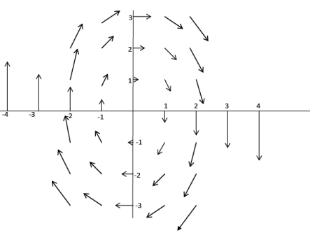
Figure 1: Graphical representation of a vector field 
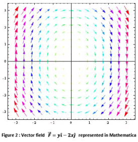
In electrostatics we deal with force field due to charges. In Fig. 3 we show the force on a unit positive charge due to two equal and opposite charges . The vector field has been plotted at close enough points so that the field lines appear continuous. To find the force on a positive charge at a point, we need to draw a tangent to the field lines at that point. These are known as “lines of force” in electrostatics”. The arrow on the lines show the direction in which the charge moves.
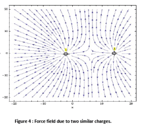
Figure 4 shows the force field due to two similar charges, a positive charge is repelled by both the charges.
Directional Derivatives :
Let me first remind you of the definition of ordinary derivative of a function f(x) of a single variable x. We define it by the relationship 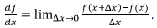 This means that the value of the function f at the point
  is its value at the point x plus the derivative of the function time the increment in the value of x. If we are given a function in one dimension, the derivative at a point is the slope of the function at that point. If the slope is positive the value of the function increases from its value at a neighbouring point, it decreases if the slope is negative.
What happens in higher dimensions? We are familiar with the concept of “partial derivative”. Suppose we have a function of x and y. The partial derivative with respect to x means that when the differentiation is done with respect to the variable x, we treat the variable y as a constant. Similarly, in taking partial derivative with respect to y, the value of x is kept fixed.
What if both x and y are to be allowed to vary simultaneously? The problem is that there are many ways the two variables can change simultaneously. Same is true for a function of three or more variables. The concept of derivative is thus to be generalized.
Suppose φ is a scalar function of the variables x, y and z. Starting from a point  if we move along an arbitrary direction by a length Δs, the value of the function at the destination
 will be given by its value at the initial point plus the derivative of the function computed along the direction in which we moved times the length Δs. Such a derivative is called the directional derivative. Since
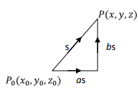
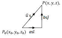
 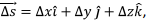 we could go from the point P0 to the point P by going by a distance Δx along the x direction, keeping y and z constant, then going by an amount along the y direction and finally by Δz along the z direction and arrive at the point P.
This is graphically shown in two dimensions :
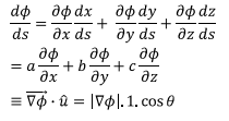
Using the definition of partial derivatives, we have,
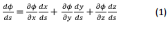
where  respectively represent the partial derivatives of φ with respect to x, y and z respectively. Equation (1) gives the directional derivative of the scalar function φ along the direction
Example : We will illustrate the concept of directional derivative by calculating the directional derivative of the scalar function 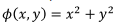 along three different directions : along
  and (ii)
  at the point (1,2).
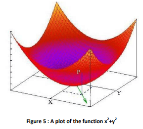
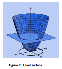
(i) The figure below shows the function plotted along the z axis. It is a cup like structure.
Since the function is in two dimensions, we have 
The partial derivatives are given by 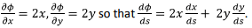 In order to calculate
  we observe that along the given direction
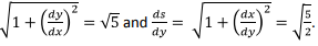
  the coordinates x and y are related by
  We have ds
 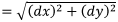 which gives
 Plugging these into the expression for
  At the point (1,2), the directional derivative
(ii) The calculation is very similar to (i). The answer is zero.
(iii) Following the method outlined in (i) above, the directional derivative at the point (1,2) can be shown to be given by  The directional derivative has a maximum when α = 2. Thus the directional derivative at (1,2) has a maximum in the direction of
  It may be noted that this is the radial direction at that point.
Suppose the direction cosines of the direction that we move is (a,b,c), the unit vector in this direction represented by  with
with  We have,
  , which gives
Which results in the directional derivative along 
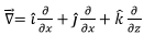
Where the “gradient operator 
where θ is the angle between the gradient and he direction in which the directional derivative is taken. Thus
(1) the magnitude of the gradient at a point is the maximum possible magnitude of the directional derivative at that point, and
(2) the direction of the gradient is that direction in which the directional derivative takes maximum value.
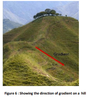
What does this physically mean? Suppose you are on a hill , not quite at the summit. If you want to come down to the base, there are many directions that you can take. Of all such possible directions, the fastest will be one which is steepest, i.e. with maximum slope.
Since the rate of change in the value of the function is maximum along the gradient, it follows that such a direction is perpendicular to a surface on which the function is constant. Such a surface is called a “Level Surface”. Returning to the function  level surface (rather a level curve in this case) is the intersection of the plane z= constant with the surface
  which are family of circles. In Physics, the corresponding surface would be an equipotential surface and the direction of the gradient would correspond to the direction of the electric field.
In the present case
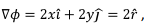 which, as expected, is in the radial direction which is normal to the level curve, which is a circle
Gradient of a Scalar Field is a Vector Field and its direction is normal to the level surface.
Formal Proof : Consider a level curve which is parameterized by a variable t, which varies from point to point on the curve. Example of such a parameter for the circle is angle θ, so that 
 where R is the radius (which is fixed) and q is the polar angle
The position vector of a point on the curve is given by  Let the level curve be given by
  The tangent to the curve is
Obviously, on the level curve 
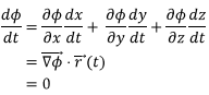
Which shows that the gradient is normal to the level curve.
|
10 videos|53 docs|56 tests
|
FAQs on Scalar Field & Its Gradient - Electromagnetic Fields Theory (EMFT) - Electrical Engineering (EE)
| 1. What is a scalar field and how is it defined? |  |
| 2. How is the gradient of a scalar field calculated? | |
| 3. What does the gradient of a scalar field represent? | |
| 4. How can the gradient of a scalar field be interpreted in physical terms? | |
| 5. What are some applications of scalar fields and their gradients in real-world scenarios? | |


Important questions
,past year papers
,MCQs
,Semester Notes
,Summary
,shortcuts and tricks
,Previous Year Questions with Solutions
,Viva Questions
,ppt
,video lectures
,practice quizzes
,Exam
,mock tests for examination
,Objective type Questions
,Extra Questions
,Sample Paper
,study material
,Scalar Field & Its Gradient | Electromagnetic Fields Theory (EMFT) - Electrical Engineering (EE)
,Free
,Scalar Field & Its Gradient | Electromagnetic Fields Theory (EMFT) - Electrical Engineering (EE)
,Scalar Field & Its Gradient | Electromagnetic Fields Theory (EMFT) - Electrical Engineering (EE)
;


Scalar Field & Its Gradient Free PDF Download
Importance of Scalar Field & Its Gradient
Scalar Field & Its Gradient Notes
Scalar Field & Its Gradient Electrical Engineering (EE) Questions
Study Scalar Field & Its Gradient on the App
|
© EduRev
|
Education Revolution
|


|


