Lecture 15 - Controller types - Electrical Engineering (EE) PDF Download

Lecture 15 -Controller types, Control Systems
If we remember the controller design in continuous domain using root locus, we see that the design is based on the approximation that the closed loop system has a complex conjugate pole pair which dominates the system behavior. Similarly for a discrete time case also the controller will be designed based on the concept of a dominant pole pair.
Controller types: We have already studied different variants of controllers such as PI, PD, PID etc. We know that PI controller is generally used to improve steady state performance whereas PD controller is used to improve the relative stability or transient response. Similarly a phase lead compensator improves the dynamic performance whereas a lag compensator improves the steady state response.
Pole-Zero cancellation A common practice in designing controllers in s-plane or z-plane is to cancel the undesired poles or zeros of plant transfer function by the zeros and poles of controller. New poles and zeros can also be added in some advantageous locations. However, one has to keep in mind that pole-zero cancellation scheme does not always provide satisfactory solution. Moreover, if the undesired poles are near j ω axis, inexact cancellation, which is almost inevitable in practice, may lead to a marginally stable or even unstable closed loop system. For this reason one should never try to cancel an unstable pole.
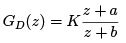
Design Procedure: Consider a compensator of the form K z + a z + b . It will be a lead com- pensator if the zero lies on the right of the pole.
1. Calculate the desired closed loop pole pairs based on design criteria.
2. Map the s-domain poles to z-domain.
3. Check if the sampling frequency is 8−10 times the desired damped frequency of oscillation.
4. Calculate the angle contributions of all open loop poles and zeros to the desired closed loop pole.
5. Compute the required contribution by the controller transfer function to satisfy angle criterion.
6. Place the controller zero in a suitable location and calculate the required angle contribution of the controller pole.
7. Compute the location of the controller pole to provide the required angle.
8. Find out the gain K from the magnitude criterion.
The following example will illustrate the design procedure.
An Example on Controller Design
Consider the closed loop discrete control system as shown in Figure 1. Design a digital controller

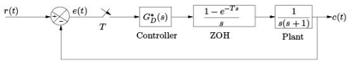
Figure 1: A discrete time control system such that the dominant closed loop poles have a damping ratio ξ = 0.5 and settling time ts = 2 sec for 2% tolerance band. Take the sampling period as T = 0.2 sec. The dominant pole pair in continuous domain is
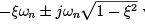 where ωn is the natural undamped frequency.
Given that settling time ts =
Thus, ωn = 4
Damped frequency ωd = 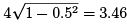
Sampling frequency ωs =
Since  = 9.07, we get approximately 9 samples per cycle of the damped oscillation.
The closed loop poles in s-plane
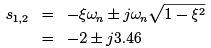
Thus the closed loop poles in z-plane
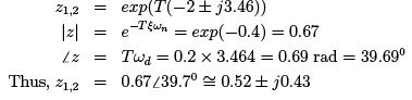
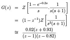
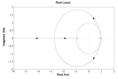
Figure 2: Root locus of uncompensated system
The root locus of the uncompensated system (without controller) is shown in Figure 2. It is clear from the root locus plot that the uncompensated system is stable for a very small range of K .
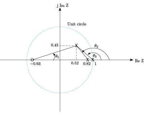
Figure 3: Pole zero map to compute angle contributions
Pole zero map of the uncompensated system is shown in Figure 3. Sum of angle contributions at the desired pole is A = θ1 − θ2 − θ3, where θ1 is the angle by the zero, −0.93, and θ2 and θ3 are the angles contributed by the two poles, 0.82 and 1 respectively.
From the pole zero map as shown in Figure 3, the angles can be calculated as θ1 = 16.5o, θ2 = 124.9o and θ3 = 138.1o.
Net angle contribution is A = 16.5o − 124.9o − 138.1o = −246.5o.
But from angle criterion a point will lie on root locus if the total angle contribution at that point is ±180o . Angle deficiency is −246.5o + 180o = −66.5o Controller pulse transfer function must provide an angle of 66.5o. Thus we need a Lead Compensator. Let us consider the following compensator.
If we place controller zero at z = 0.82 to cancel the pole there, we can avoid some of the calculations involved in the design. Then the controller pole should provide an angle of 124.9o − 66.5o = 58.4o.
Once we know the required angle contribution of the controller pole, we can easily calculate the pole location as follows.
The pole location is already assumed at z = −b. Since the required angle is greater than tan−1(0.43/0.52) = 39.6o we can easily say that the pole must lie on the right half of the unit circle. Thus b should be negative. To satisfy angle criterion,
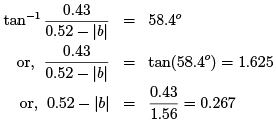
Thus, b = −0.253
The controller is then written as GD (z) = .The root locus of the compensated
system (with controller) is shown in Figure 4.
If we compare Figure 4 with Figure 2, it is evident that stable region of K is much larger for the compensated system than the uncompensated system. Next we need to calculate K from the magnitude criterion.
Magnitude criterion :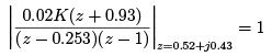
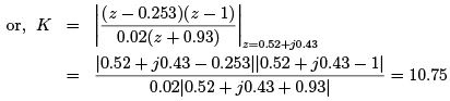
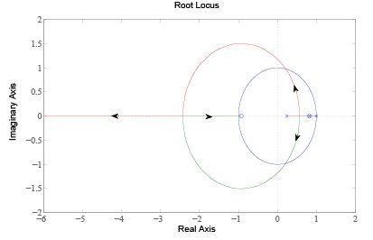
Figure 4: Root locus of the compensated system
Thus the required controller is GD (z) = 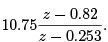 The SIMULINK block to compute the output response is shown in Figure 5. All discrete blocks in the SIMULINK model should have same sampling period which is 0.2 sec in this example. The scope output is shown in Figure 6.

Figure 5: Simulink diagram of the closed loop system
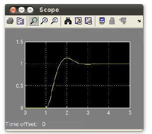
Figure 6: Output response of the closed loop system
FAQs on Lecture 15 - Controller types - Electrical Engineering (EE)
| 1. What are the different types of controllers? |  |
| 2. How does a proportional controller work? | |
| 3. What is an integral controller? | |
| 4. How does a derivative controller work? | |
| 5. What is a PID controller? | |


Top Courses for Electrical Engineering (EE)

Free
,Semester Notes
,practice quizzes
,Summary
,Viva Questions
,Exam
,past year papers
,Objective type Questions
,video lectures
,Previous Year Questions with Solutions
,Sample Paper
,Lecture 15 - Controller types - Electrical Engineering (EE)
,Important questions
,ppt
,study material
,Lecture 15 - Controller types - Electrical Engineering (EE)
,mock tests for examination
,MCQs
,Extra Questions
,shortcuts and tricks
,Lecture 15 - Controller types - Electrical Engineering (EE)
;


Lecture 15 - Controller types Free PDF Download
Importance of Lecture 15 - Controller types
Lecture 15 - Controller types Notes
Lecture 15 - Controller types Electrical Engineering (EE) Questions
Study Lecture 15 - Controller types on the App
|
© EduRev
|
Education Revolution
|


|


within 7 days!