Lecture 25 - Introduction to State Variable Model - Electrical Engineering (EE) PDF Download

Lecture 25 - Introduction to State Variable Model, Control Systems
1 Introduction to State Variable Model
In the preceding lectures, we have learned how to design a sampled data control system or a digital system using the transfer function of the system to be controlled. Transfer function approach of system modeling provides final relation between output variable and input variable.
However, a system may have other internal variables of importance. State variable representation takes into account of all such internal variables. Moreover, controller design using classical methods, e.g., root locus or frequency domain method are limited to only LTI systems, particularly SISO (single input single output) systems since for MIMO (multi input multi output) systems controller design using classical approach becomes more complex. These limitations of classical approach led to the development of state variable approach of system modeling and control which formed a basis of modern control theory.
State variable models are basically time domain models where we are interested in the dynamics of some characterizing variables called state variables which along with the input represent the state of a system at a given time.
- State: The state of a dynamic system is the smallest set of variables, x ∈ Rn, such that given x(t0) and u(t), t > t0, x(t), t > t0 can be uniquely determined.
- Usually a system governed by a nth order differential equation or nth order transfer function is expressed in terms of n state variables: x1 , x2 , . . . , xn
- The generic structure of a state-space model of a nth order continuous time dynamical system with m input and p output is given by:
x˙ (t) = Ax(t) + B u(t) : State Equation (1)
y(t) = C x(t) + Du(t) : Output Equation
where, x(t) is the n dimensional state vector, u(t) is the m dimensional input vector, y(t) is the p dimensional output vector and A ∈ Rn×n, B ∈ Rn×m, C ∈ Rp×n, D ∈ Rp×m.
Example
Consider a nth order differential equation

Define following variables,
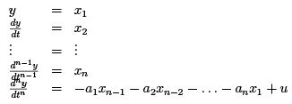
The nth order differential equation may be written in the form of n first order differential equations as
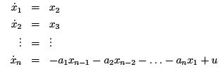
or in matrix form as,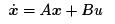
where

The output can be one of states or a combination of many states. Since, y = x1,
y = [1 0 0 0 . . . 0]x
1.1 Correlation between state variable and transfer functions models
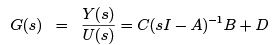
The transfer function corresponding to state variable model (1), when u and y are scalars, is:
 (2)
(2)
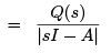
where |sI − A| is the characteristic polynomial of the system.
1.2 Solution of Continuous
Time State Equation The solution of state equation (1) is given as
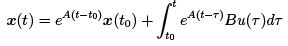
where eAt = Φ(t) is known as the state transition matrix and x(t0) is the initial state of the system.
2 State Variable Analysis of Digital Control Systems
The discrete time systems, as discussed earlier, can be classified in two types.
1. Systems that result from sampling the continuous time system output at discrete instants only, i.e., sampled data systems.
2. Systems which are inherently discrete where the system states are defined only at discrete time instants and what happens in between is of no concern to us.
2.1 State Equations of Sampled Data Systems
Let us assume that the following continuous time system is sub ject to sampling process with an interval of T .
x˙ (t) = Ax(t) + B u(t) : State Equation (3)
y(t) = C x(t) + Du(t) : Output Equation
We know that the solution to above state equation is:
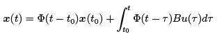
Since the inputs are constants in between two sampling instants, one can write:
u(τ ) = u(kT ) for, kT ≤ τ ≤ (k + 1)T
which implies that the following expression is valid within the interval kT ≤ τ ≤ (k + 1)T if we consider t0 = kT :
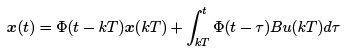
Let us denote 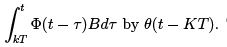 Then we can write:
x(t) = Φ(t − kT )x(kT ) + θ(t − K T )u(kT )
If t = (k + 1)T ,
x((k + 1)T ) = Φ(T )x(kT ) + θ(T )u(kT ) (4)
where 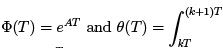 Φ((k + 1)T − τ )B dτ . If t' = τ − kT , we can rewrite
 Equation (4) has a similar form as that of equation (3) if we consider φ(T ) =
  and θ(T ) =
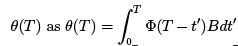
  . Similarly by setting t = kT , one can show that the output equation also has a similar form as that of the continuous time one.
When T = 1,
x(k + 1) = Φ(1)x(k) + θ(1)u(k) y(k) = C x(k) + Du(k)
2.2 State Equations of Inherently Discrete Systems
When a discrete system is composed of all digital signals, the state and output equations can be described by
x(k + 1) = Ax(k) + Bu(k)
y(k) = C x(k) + Du(k)
2.3 Discrete Time Approximation of A Continuous Time State Space Model
Let us consider the dynamical system described by the state space model (3). By approximating the derivative at t = kT using forward difference, we can write:
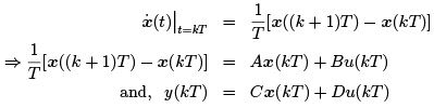
Rearranging the above equations,
x((k + 1)T ) = (I + T A)x(kT ) + T Bu(kT )
If, T = 1 ⇒ x(k + 1) = (I + A)x(k) + Bu(k)
and y(k) = C x(k) + Du(k)
We can thus conclude from the discussions so far that the discrete time state variable model of a system can be described by
x(k + 1) = Ax(k) + Bu(k)
y(k) = C x(k) + Du(k)
where A, B are either the descriptions of an all digital system or obtained by sampling the continuous time process.
FAQs on Lecture 25 - Introduction to State Variable Model - Electrical Engineering (EE)
| 1. What is a state variable model? |  |
| 2. How is a state variable model different from other modeling techniques? | |
| 3. What are the advantages of using a state variable model? | |
| 4. How do you derive a state variable model from a physical system? | |
| 5. What are some common applications of state variable models? | |


Top Courses for Electrical Engineering (EE)

practice quizzes
,Semester Notes
,past year papers
,study material
,Lecture 25 - Introduction to State Variable Model - Electrical Engineering (EE)
,shortcuts and tricks
,ppt
,Lecture 25 - Introduction to State Variable Model - Electrical Engineering (EE)
,Sample Paper
,mock tests for examination
,Important questions
,Viva Questions
,Free
,MCQs
,Previous Year Questions with Solutions
,Lecture 25 - Introduction to State Variable Model - Electrical Engineering (EE)
,video lectures
,Summary
,Exam
,Extra Questions
,Objective type Questions
;


Lecture 25 - Introduction to State Variable Model Free PDF Download
Importance of Lecture 25 - Introduction to State Variable Model
Lecture 25 - Introduction to State Variable Model Notes
Lecture 25 - Introduction to State Variable Model Electrical Engineering (EE) Questions
Study Lecture 25 - Introduction to State Variable Model on the App
|
© EduRev
|
Education Revolution
|


|


within 7 days!