Lecture 26 - State Space Model to Transfer Function - Electrical Engineering (EE) PDF Download

Lecture 26 - State Space Model to Transfer Function, Control Systems
In this lecture we will discuss about the relation between transfer function and state space model for a discrete time system and various standard or canonical state variable models.
1 State Space Model to Transfer Function
Consider a discrete state variable model
x(k + 1) = Ax(k) + Bu(k)
y(k) = C x(k) + Du(k) (1)
Taking the Z-transform on both sides of Eqn. (1), we get
zX (z) − zx0 = AX (z) + BU (z)
Y (z) = C X (z) + DU (z)
where x0 is the initial state of the system.
⇒ (zI − A)X (z) = zx0 + BU (z)
or, X (z) = (zI − A)−1zx0 + (zI − A)−1B U (z)
To find out the transfer function, we assume that the initial conditions are zero, i.e., x0 = 0, thus
Y (z) = (C (zI − A)−1B + D)U (z)
Therefore, the transfer function becomes
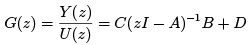 (2)
(2)
which has the same form as that of a continuous time system.
2 Various Canonical Forms
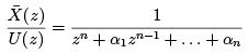
We have seen that transform domain analysis of a digital control system yields a transfer function of the following form.
 (3)
(3)
Various canonical state variable models can be derived from the above transfer function model.
2.1 Controllable canonical form
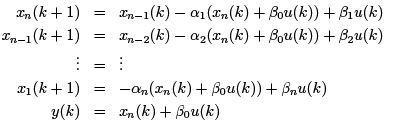
Consider the transfer function as given in Eqn. (3). Without loss of generality, let us consider the case when m = n. Let
In time domain, the above equation may be written as

Now, the output Y (z) may be written in terms of  as
as
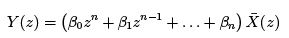
or in time domain as

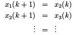
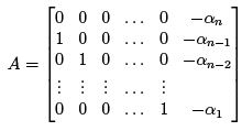
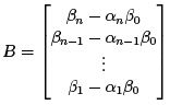
The block diagram representation of above equations is shown in Figure 1. State variables are selected as shown in Figure 1.
The state equations are then written as:

Output equation can be written as by following the Figure 1.
y(k) = (βn − αnβ0)x1(k) + (βn−1 − αn−1β0)x2(k) + . . . + (β1 − α1β0)xn(k) + β0u(k)
In state space form, we have
x(k + 1) = Ax(k) + Bu(k)
y(k) = C x(k) + Du(k) (4)
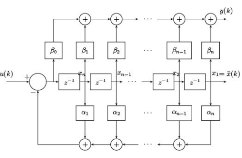
Figure 1: Block Diagram representation of controllable canonical form
where
2.2 Observable Canonical Form
Equation (3) may be rewritten as
The corresponding block diagram is shown in Figure 2. Choosing the outputs of the delay blocks
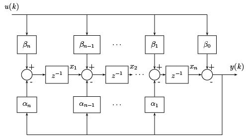
Figure 2: Block Diagram representation of observable canonical form as the state variables, we have following state equations
This can be rewritten in matrix form (4) with
 C = [0 0 . . . 1] D = β0
2.3 Duality
In previous two sections we observed that the system matrix A in observable canonical form is transpose of the system matrix in controllable canonical form. Similarly, control matrix B in observable canonical form is transpose of output matrix C in controllable canonical form. So also output matrix C in observable canonical form is transpose of control matrix B in controllable canonical form.
2.4 Jordan Canonical Form
In Jordan canonical form, the system matrix A represents a diagonal matrix for distinct poles which basically form the diagonal elements of A.
Assume that z = λi, i = 1, 2, . . . , n are the distinct poles of the given transfer function (3). Then partial fraction expansion of the transfer function yields
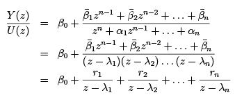 (5)
(5)
A parallel realization of the transfer function (5) is shown in Figure 3.
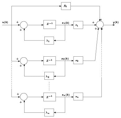
Figure 3: Block Diagram representation of Jordan canonical form
Considering the outputs of the delay blocks as the state variables, we can construct the state model in matrix form (4), with
 C = [r1 r2 . . . rn] D = β0
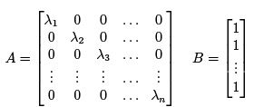
When the matrix A has repeated eigenvalues, it cannot be expressed in a proper diagonal form.
However, it can be expressed in a Jordan canonical form which is nearly a diagonal matrix. Let us consider that the system has eigenvalues, λ1, λ1, λ2 and λ3. In that case, A matrix in Jordan canonical form will be
1. The diagonal elements of the matrix A are eigenvalues of the same.
2. The elements below the principal diagonal are zero.
3. Some of the elements just above the principal diagonal are one.
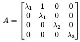
4. The matrix can be divided into a number of blocks, called Jordan blocks, along the diagonal. Each block depends on the multiplicity of the eigenvalue associated with it. For example Jordan block associated with a eigenvalue z1 of multiplicity 4 can be written as
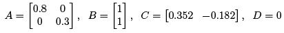
Example: Consider the following discrete transfer function.
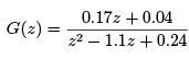
Find out the state variable model in 3 different canonical forms.
Solution: The state variable model in controllable canonical form can directly be derived from the transfer function, where the A, B , C and D matrices are as follows:
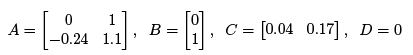
The matrices in state model corresponding to observable canonical form are obtained as,
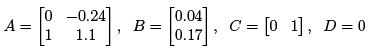
To find out the state model in Jordan canonical form, we need to fact expand the transfer function using partial fraction, as
FAQs on Lecture 26 - State Space Model to Transfer Function - Electrical Engineering (EE)
| 1. What is a state space model? |  |
| 2. How can a state space model be converted to a transfer function? | |
| 3. What advantages does a state space model offer over a transfer function? | |
| 4. What are the limitations of using state space models? | |
| 5. Can a transfer function be converted back to a state space model? | |


Top Courses for Electrical Engineering (EE)

shortcuts and tricks
,ppt
,Extra Questions
,Free
,Objective type Questions
,past year papers
,Summary
,Viva Questions
,Important questions
,Semester Notes
,Sample Paper
,Lecture 26 - State Space Model to Transfer Function - Electrical Engineering (EE)
,Previous Year Questions with Solutions
,practice quizzes
,video lectures
,Exam
,MCQs
,study material
,mock tests for examination
,Lecture 26 - State Space Model to Transfer Function - Electrical Engineering (EE)
,Lecture 26 - State Space Model to Transfer Function - Electrical Engineering (EE)
;


Lecture 26 - State Space Model to Transfer Function Free PDF Download
Importance of Lecture 26 - State Space Model to Transfer Function
Lecture 26 - State Space Model to Transfer Function Notes
Lecture 26 - State Space Model to Transfer Function Electrical Engineering (EE) Questions
Study Lecture 26 - State Space Model to Transfer Function on the App
|
© EduRev
|
Education Revolution
|


|


