Lecture 28 - Solution to Discrete State Equation | 6 Months Preparation for GATE Electrical - Electrical Engineering (EE) PDF Download

Lecture 28 - Solution to Discrete State Equation, Control Systems
1 Solution to Discrete State Equation
Consider the following state model of a discrete time system: x(k + 1) = Ax(k) + Bu(k) where the initial conditions are x(0) and u(0). Putting k = 0 in the above equation, we get
x(1) = Ax(0) + Bu(0)
Similarly if we put k = 1, we would get
x(2) = Ax(1) + Bu(1)
Putting the expression of x(1) ⇒ x(2) = A2x(0) + AB u(0) + B u(1)
For k = 2,
x(3) = Ax(2) + Bu(2)
= A3x(0) + A2Bu(0) + ABu(1) + Bu(2) and so on.
If we combine all these equations, we would get the following expression as a general solution:
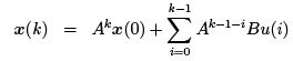
As seen in the above expression, x(k) has two parts. One is the contribution due to the initial state x(0) and the other one is the contribution of the external input u(i) for i = 0, 1, 2, · · · , k −1.
When the input is zero, solution of the homogeneous state equation x(k + 1) = Ax(k) can be written as
x(k) = Ak x(0)
where Ak = φ(k) is the state transition matrix.
2 Evaluation of φ(k)
Similar to the continuous time systems, the state transition matrix of a discrete state model can be evaluated using the following different techniques.
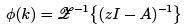
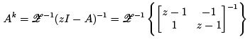
1. Using Inverse Z-transform:
2. Using Similarity Transformation If Λ is the diagonal representation of the matrix A, then Λ = P −1AP . When a matrix is in diagonal form, computation of state transition matrix is straight forward:
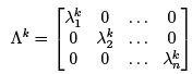
Given Λk , we can compute Ak = P Λk P −1
3. Using Caley Hamilton Theorem
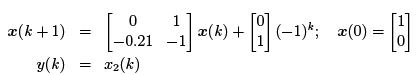
Example Compute Ak for the following system using three different techniques and hence find y(k) for k ≥ 0.
Solution: A =  and eigenvalues of A are −0.3 and −0.7.
Method 1

Method 2
Ak = P Λk P −1 where Λk =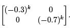 Eigen values are −0.3 and −0.7. The corresponding eigenvectors are found, by using equation Avi = λivi, as
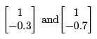 respectively. The transformation matrix is given by

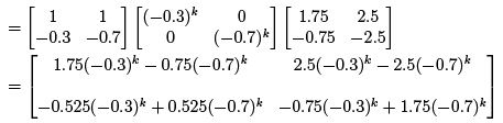
Thus,
Ak = P ΛkP −1
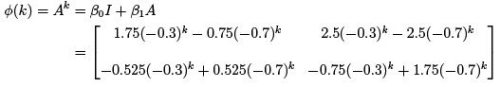
Method 3: Caley Hamilton Theorem
The eigenvalues are −0.3 and −0.7
(−0.3)k = β0 − 0.3β1
(−0.7)k = β0 − 0.7β1
Solving,
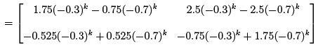
β0 = 1.75(−0.3)k − 0.75(−0.7)k
β1 = 2.5(−0.3)k − 2.5(−0.7)k
Hence,
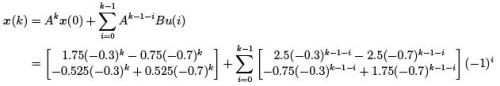
The solution x(k) is
Since y(k) = x2(k), we can write
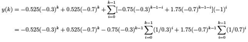
Now,
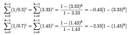
Putting the above expression in y(k)
y(k) = 0.475(−0.3)k − 5.3(−0.7)k + (−0.3)k (3.33)k + 5.825(−0.7)k−1(1.43)k
3 State Diagram
Conventional signal flow graph method was meant for only algebraic equation, thus these are generally used for the derivation of input output relation in a transformed domain.
State diagram or state transition signal flow graph is an extension of conventional signal flow graph which can be applied to represent differential and difference equations as well.
Example 1: Draw the state diagram for the following differential equation.
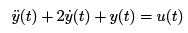
Considering the state variables as x1(t) = y(t) and x2(t) =  , we can write
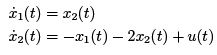
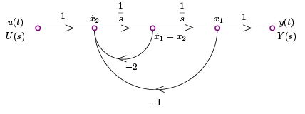
Figure 1: State Diagram of Example 1
The state diagram is shown in Figure 1.
Example 2: Consider a discrete time system described by the following state difference equations.
x1(k + 1) = −x1(k) + x2(k)
x2(k + 1) = −x1(k) + u(k)
y(k) = x1(k) + x2(k)
Draw the state diagram.
The state diagram is shown in Figure 2.
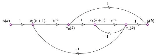
Figure 2: State Diagram of Example 2
3.1 State Diagram of Zero Order Hold
State diagram of zero order hold is important for sampled date control systems. Let the input to and output of a ZOH is e∗(t) and h(t) respectively. Then, for the inetrval kT ≤ t ≤
(k + 1)T , h(t)e(kT )
Or,
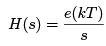
Therefore, the state diagram, as shown in Figure 3, consists of a single branch with gain s−1.
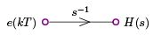
Figure 3: State Diagram of Zero Order Hold
4 System Response between Sampling Instants
State variable method is a convenient way to evaluate the system response between the sampling instants of a sampled data system. State transition equation is given as:
where x(t0) is the initial state of the system and u(t) is the external input.
when t0 = kT , x(t) = φ(t − kT )x(kT ) + u(kT )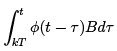
Since we are interested in response between the sampling instants, let us consider t = (k + ∆)T where k = 0, 1, 2, · · · and 0 ≤ ∆ ≤ 1. This implies
x((k + ∆)T ) = φ(∆T )x(kT ) + θ(∆T )u(kT )
where 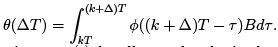 By varying the value of ∆ between 0 and 1 all information on x(t) for all t can be obtained.
Example 3: Consider the following state model of a continuous time system.
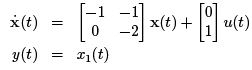
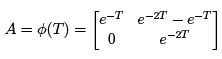
which undergoes through a sampling process with period T . To derive the discrete state space model, let us first compute the state transition matrix of the continuous time system using Caley Hamilton Theorem.

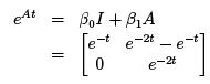
Let f (λ) = eλt
This implies
e−t = β0 − β1 (λ1 = −1)
e−2t = β0 − 2β1 (λ2 = −2)
Solving the above equations
β1 = e−t − e−2t β0 = 2e−t − e−2t
Then
Thus the discrete state matrix A is given as
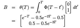
The discrete input matrix B can be computed as
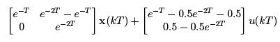
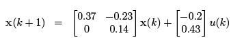
When t = (k + 1)T , the discrete state equation is described by
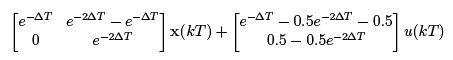
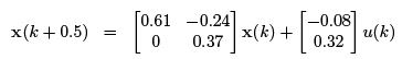
When t = (k + ∆)T ,
If the sampling period T = 1,
At the sampling instants we can find x(k) by putting k = 0, 1, 2 · · · . If ∆ = 0.5, then between the sampling instants,
The responses in between the sampling instants, i.e., x(0.5), x(1.5), x(2.5) etc., can be found by putting k = 0, 1, 2 · · · .
|
675 videos|1315 docs|882 tests
|
FAQs on Lecture 28 - Solution to Discrete State Equation - 6 Months Preparation for GATE Electrical - Electrical Engineering (EE)
| 1. What is a discrete state equation? |  |
| 2. How is a discrete state equation solved? | |
| 3. What are the applications of discrete state equations? | |
| 4. Can discrete state equations be used to model real-world systems accurately? | |
| 5. Are there any limitations or challenges in solving discrete state equations? | |


MCQs
,Exam
,Sample Paper
,practice quizzes
,Objective type Questions
,mock tests for examination
,Lecture 28 - Solution to Discrete State Equation | 6 Months Preparation for GATE Electrical - Electrical Engineering (EE)
,Semester Notes
,study material
,Free
,Summary
,Previous Year Questions with Solutions
,ppt
,Important questions
,Lecture 28 - Solution to Discrete State Equation | 6 Months Preparation for GATE Electrical - Electrical Engineering (EE)
,past year papers
,Extra Questions
,Lecture 28 - Solution to Discrete State Equation | 6 Months Preparation for GATE Electrical - Electrical Engineering (EE)
,Viva Questions
,shortcuts and tricks
,video lectures
;


Lecture 28 - Solution to Discrete State Equation Free PDF Download
Importance of Lecture 28 - Solution to Discrete State Equation
Lecture 28 - Solution to Discrete State Equation Notes
Lecture 28 - Solution to Discrete State Equation Electrical Engineering (EE) Questions
Study Lecture 28 - Solution to Discrete State Equation on the App
|
© EduRev
|
Education Revolution
|


|


