Lecture 29 - Controllability - Electrical Engineering (EE) PDF Download

Lecture 29 - Controllability, Control Systems
Controllability and observability are two important properties of state models which are to be studied prior to designing a controller.
Controllability deals with the possibility of forcing the system to a particular state by application of a control input. If a state is uncontrollable then no input will be able to control that state. On the other hand whether or not the initial states can be observed from the output is determined using observability property. Thus if a state is not observable then the controller will not be able to determine its behavior from the system output and hence not be able to use that state to stabilize the system.
1 Controllability
Before going to any details, we would first formally define controllability. Consider a dynamical system
x(k + 1) = Ax(k) + Bu(k) (1)
y(k) = C x(k) + Du(k)
where A ∈ Rn×n, B ∈ Rn×m, C ∈ Rp×n, D ∈ Rp×m.
Definition 1. Complete State Controllability: The state equation (1) (or the pair (A, B ) ) is said to be completely state control lable or simply state control lable if for any initial state x(0) and any final state x(N ), there exists an input sequence u(k), k = 0, 1, 2, · · · , N , which transfers x(0) to x(N ) for some finite N . Otherwise the state equation (1) is state uncontrol lable.
Definition 2. Complete Output Controllability: The system given in equation (1) is said to be completely output control lable or simply output control lable if any final output y(N ) can be reached from any initial state x(0) by applying an unconstrained input sequence u(k), k = 0, 1, 2, · · · , N , for some finite N . Otherwise (1) is not output control lable.
1.1 Theorems on controllability
State Controllability: 1. The state equation (1) or the pair (A, B ) is state controllable if and only if the n × nm state controllability matrix
UC = ]B AB A2B ...... An−1B ]
has rank n i.e., full row rank.
2. The state equation (1) is controllable if the n × n controllability grammian matrix

is non-singular for any nonzero finite N .
3. If the system has a single input and the state model is in controllable canonical form then the system is controllable.
4. When A has distinct eigenvalues and in Jordan/Diagonal canonical form, the state model is controllable if and only if all the rows of B are nonzero.
5. When A has multiple order eigenvalues and in Jordan canonical form, then the state model is controllable if and only if
i. each Jordan block corresponds to one distinct eigenvalue and
ii. the elements of B that correspond to last row of each Jordan block are not all zero.
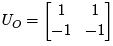
Output Controllability: The system in equation (1) is completely output controllable if and only if the p × (n + 1)m output controllability matrix
UOC = [D C B C AB C A2B ...... C An−1B] has rank p, i.e., full row rank.
1.2 Controllability to the origin and Reachability
There exist three different definitions of state controllability in the literature:
1. Input transfers any state to any state. This definition is adopted in this course.
2. Input transfers any state to zero state. This is called controllability to the origin.
3. Input transfers zero state to any state. This is referred as controllability from the origin or reachability.
Above three definitions are equivalent for continuous time system. For discrete time systems definitions (1) and (3) are equivalent but not the second one.
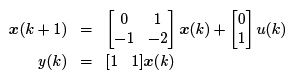
Example: Consider the system x(k + 1) = Ax(k) + B u(k), y(k) = C x(k). where
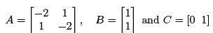
Show if the system is controllable. Find the transfer function  Can you see any connection between controllability and the transfer function?
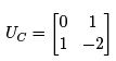
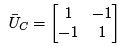
Solution: The controllability matrix is given by
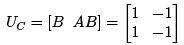
Its determinant  has a rank 1 which is less than the order of the matrix, i.e., 2.
Thus the system is not controllable. The transfer function
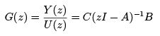
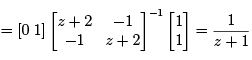
Although state model is of order 2, the transfer function has order 1. The eigenvalues of A are λ1 = −1 and λ2 = −3. This implies that the transfer function is associated with pole-zero cancellation for the pole at −3. Since one of the dynamic modes is cancelled, the system became uncontrollable.
2 Observability
Definition 3. The state model (1) (or the pair (A, C ) ) is said to be observable if any initial state x(0) can be uniquely determined from the know ldge of output y(k) and input sequence u(k), for k = 0, 1, 2, · · · , N , where N is some finite time. Otherwise the state model (1) is unobservable.
2.1 Theorems on observability
1. The state model (1) or the pair (A, C ) is observable if the np × n observability matrix
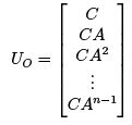
has rank n, i.e., full column rank.
2. The state model (1) is observable if the n × n observability grammian matrix
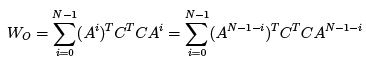
is non-singular for any nonzero finite N .
3. If the state model is in observable canonical form then the system is observable.
4. When A has distinct eigenvalues and in Jordan/Diagonal canonical form, the state model is observable if and only if none of the columns of C contain zeros.
5. When A has multiple order eigenvalues and in Jordan canonical form, then the state model is observable if and only if i. each Jordan block corresponds to one distinct eigenvalue and ii. the elements of C that correspond to first column of each Jordan block are not all zero.
2.2 Theorem of Duality The pair (A, B ) is control lable if and only if the pair (AT , B T ) is observable.
Exercise: Prove the theorem of duality.
3 Loss of controllability or observability due to pole-zero cancellation
We have already seen through an example that a system becomes uncontrollable when one of the modes is cancelled. Let us take another example.
Example:
The controllability matrix
implies that the state model is controllable. On the other hand, the observability matrix
has a rank 1 which implies that the state model is unobservable. Now, if we take a different set of state variables so that,  (k) = y(k), then the state variable model will be:
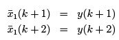 = −y(k) − 2y(k + 1) + u(k + 1) + u(k)
Lets us take  (k) = y(k + 1) − u(k). The new state variable model is:
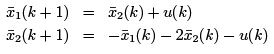
which implies
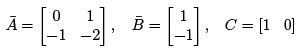
The controllability matrix
implies that the state model is uncontrollable. The observability matrix

implies that the state model is observable. The system difference equation will result in a transfer function which would involve pole-zero cancellation. Whenever there is a pole zero cancellation, the state space model will be either uncontrollable or unobservable or both.
4 Controllability/Observability after sampling
Question: If a continuous time system is undergone a sampling process will its controllability or observability property be maintained?
The answer to the question depends on the sampling period T and the location of the eigenvalues of A.
- Loss of controllability and/or observability occurs only in presence of oscillatory modes of the system.
- A sufficient condition for the discrete model with sampling period T to be controllable is that whenever
 for m = 1, 2, 3, ...
 - The above is also a necessary condition for a single input case.
Note: If a continuous time system is not control lable or observable, then its discrete time version, with any sampling period, is not control lable or observable.
FAQs on Lecture 29 - Controllability - Electrical Engineering (EE)
| 1. What is controllability in the context of lecture 29? |  |
| 2. How is controllability determined in a system? | |
| 3. Why is controllability important in engineering and control systems? | |
| 4. What are some factors that affect the controllability of a system? | |
| 5. Can a system be uncontrollable? | |


Top Courses for Electrical Engineering (EE)

Objective type Questions
,past year papers
,Free
,video lectures
,Previous Year Questions with Solutions
,Sample Paper
,Lecture 29 - Controllability - Electrical Engineering (EE)
,Lecture 29 - Controllability - Electrical Engineering (EE)
,study material
,mock tests for examination
,Summary
,MCQs
,Extra Questions
,Lecture 29 - Controllability - Electrical Engineering (EE)
,Viva Questions
,ppt
,shortcuts and tricks
,Semester Notes
,Important questions
,practice quizzes
,Exam
;


Lecture 29 - Controllability Free PDF Download
Importance of Lecture 29 - Controllability
Lecture 29 - Controllability Notes
Lecture 29 - Controllability Electrical Engineering (EE) Questions
Study Lecture 29 - Controllability on the App
|
© EduRev
|
Education Revolution
|


|


