
Best Study Material for Electrical Engineering (EE) Exam
Electrical Engineering (EE) Exam > Electrical Engineering (EE) Notes > Lecture 31 - Revisiting the Basics Linearization of A Nonlinear System Consider a System
Lecture 31 - Revisiting the Basics Linearization of A Nonlinear System Consider a System - Electrical Engineering (EE) PDF Download
Lecture 31 -Revisiting the basics Linearization of A Nonlinear System Consider a system, Control Systems
In this lecture we would discuss Lyapunov stability theorem and derive the Lyapunov Matrix Equation for discrete time systems.
1 Revisiting the basics
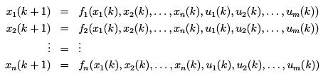
Linearization of A Nonlinear System Consider a system
x(k + 1) = f (x(k), u(k))
where functions fi(.) are continuously differentiable. The equilibrium point (xe, ue) for this system is defined as
f (xe, ue) = 0
- What is linearization?
Linearization is the process of replacing the nonlinear system model by its linear counterpart in a small region about its equilibrium point.
- Why do we need it?
We have well stabilised tools to analyze and stabilize linear systems.
The method: Let us write the general form of nonlinear system  = f (x, u) as:
Let 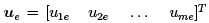 be a constant input that forces the system to settle into a constant equilibrium state xe = [x1e x2e . . . xne]T such that f (xe, ue) = 0 holds true.
We now perturb the equilibrium state by allowing: x = xe +∆x and u = ue +∆u. Taylor’s expansion yields
∆x(k + 1) = f (xe + ∆x, ue + ∆u) = f (xe, ue)
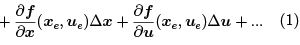
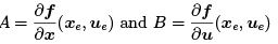
where
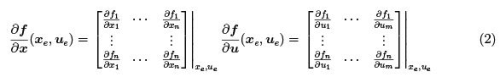
are the Jacobian matrices of f with respect to x and u, evaluated at the equilibrium point, 
Note that f (xe, ue) = 0. Let
 (3)
(3)
Neglecting higher order terms, we arrive at the linear approximation
∆x(k + 1) = A∆x(k) + B∆u(k) (4)
Similarly, if the outputs of the nonlinear system model are of the form
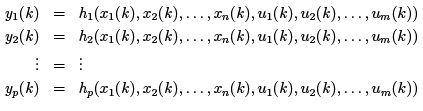
or in vector notation y(k) = h(x(k), u(k)) (5)
then Taylor’s series expansion can again be used to yield the linear approximation of the above output equations. Indeed, if we let
y = ye + ∆y (6)
then we obtain
∆y(k) = C ∆x(k) + D∆u(k) (7)
Example: Consider a nonlinear system
 (8a)
(8a)
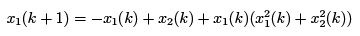 (8b)
(8b)
Linearize the system about origin which is an equilibrium point.
Evaluating the coefficients of Eqn. (3), we get
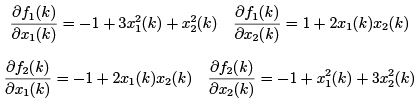
Thus 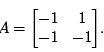 Hence, the linearized system around origin is given by
 (9)
(9)
Sign definiteness of functions and matrices
Positive Definite Function: A continuously differentiable function f : Rn → R+ is said to be positive definite in a region S ∈ Rn that contains the origin if
1. f (0) = 0
2. f (x) > 0; x ∈ S and x = 0
The function f (x) is said to be positive semi-definite
1. f (0) = 0
2. f (x) ≥ 0; x ∈ S and x = 0
If the condition (2) becomes f (x) < 0, the function is negative definite and if it becomes f (x) ≤ 0 it is negative semi-definite.
Example: Is the function f (x1, x2) =  positive definite?
Answer: f (0, 0) = 0 shows that the first condition is satisfied. f (x1, x2) > 0 for x1, x2 = 0.
Second condition is also satisfied. Hence the function is positive definite.
A square matrix P is symmetric if P = PT . A scalar function has a quadratic form if it can be written as xT P x where P = PT and x is any real vector of dimension n × 1.
Positive Definite Matrix: A real symmetric matrix P is positive definite, i.e. P > 0 if
1. xT P x > 0 for every non-zero x.
2. xT P x = 0 only if x = 0.
A real symmetric matrix P is positive semi-definite, i.e. P ≥ 0 if xT P x ≥ 0 for every non-zero x. This implies that xT P x = 0 for some x  0.
0.
Theorem: A symmetric square matrix P is positive definite if and only if any one of the following conditions holds.
1. Every eigenvalue of P is positive.
2. All the leading principal minors of P are positive.
3. There exists an n × n non-singular matrix Q such that P = QT Q.
Similarly, a matrix P is said to be negative definite if −P is positive definite. When none of these two conditions satisfies, the definiteness of the matrix cannot be calculated or in other words it is said to be sign indefinite.
Example: Consider the following third order matrices. Determine the sign definiteness of them.
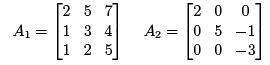
The leading principal minors of the matrix A1 are 2, 1 and 2, hence the matrix is positive definite.
The eigenvalues of the matrix A2 can be straightaway computed as 2, 5 and −3, i.e., all the eigenvalues are not positive. Again, the eigenvalues of the matrix −A2 are −2, −5 and 3 and hence the matrix A2 is sign indefinite.
2 Lyapunov Stability
Theorems In the last section we have discussed various stability definitions. But the big question is how do we determine or check the stability or instability of an equilibrium point?
Lyapunov introduced two methods.
The first is called Lyapunov’s first or indirect method: we have already seen it as the linearization technique. Start with a nonlinear system
x(k + 1) = f (x(k)) (10)
Expanding in Taylor series around xe and neglecting higher order terms.
∆x(k + 1) = A∆x(k) (11)
where (12)
(12)
Then the nonlinear system (10) is asymptotically stable around xe if and only if the linear system (11) is; i.e., if all eigenvalues of A are inside the unit circle.
The above method is very popular because it is easy to apply and it works well for most systems, all we need to do is to be able to evaluate partial derivatives.
One disadvantage of the method is that if some eigenvalues of A are on the unit circle and the rest are inside the unit circle, then we cannot draw any conclusions, the equilibrium can be either stable or unstable.
The ma jor drawback, however, is that since it involves linearization it is applied for situations when the initial conditions are “close” to the equilibrium. The method provides no indication as to how close is “close”, which may be extremely important in practical applications.
The second method is Lyapunov’s second or direct method: this is a generalization of Lagrange’s concept of stability of minimum potential energy.
Consider the nonlinear system (10). Without loss of generality, we assume origin as the equilibrium point of the system. Suppose that there exists a function, called ‘Lyapunov function’, V (x) with the following properties:
1. V (0) = 0
2. V (x) > 0, for x = 0
3. ∆V (x) < 0 along tra jectories of (10).
Then, origin is asymptotically stable.
We can see that the method hinges on the existence of a Lyapunov function, which is an energy-like function, zero at equilibrium, positive definite everywhere else, and continuously decreasing as we approach the equilibrium.
The method is very powerful and it has several advantages:
- answers questions of stability of nonlinear systems
- can easily handle time varying systems
- determines asymptotic stability as well as normal stability
- determines the region of asymptotic stability or the domain of attraction of an equilibrium The main drawback of the method is that there is no systematic way of obtaining Lyapunov functions, this is more of an art than science.
Lyapunov Matrix Equation It is also possible to find a Lyapunov function for a linear system. For a linear system of the form x(k + 1) = Ax(k) we choose as Lyapunov function the quadratic form
V (x(k)) = xT (k)P x(k) (13)
where P is a symmetric positive definite matrix. Thus
∆V (x(k)) = V (x(k + 1)) − V (x(k)) = x(k + 1)T P x(k + 1) − xT (k)P x(k) (14)
Simplifying the above equation and omitting k
∆V (x) = (Ax)T P Ax − xT P x
= xT AT P Ax − xT P x (15)
= xT (AT P A − P )x
= −xT Qx
where
AT P A − P = −Q (16)
If the matrix Q is positive definite, then the system is asymptotically stable. Therefore, we could pick Q = I , the identity matrix and solve
AT P A − P = −I
for P and see if P is positive definite.
The equation (16) is called Lyapunov’s matrix equation for discrete time systems and can be solved through MATLAB by using the command dlyap.
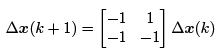
Example: Determine the stability of the following system by solving Lyapunov matrix equation
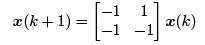
Let us take 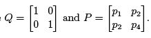 Putting these into Lyapunov matrix equation,
Thus
2p2 + p4 = −1
−p1 + p4 − p2 = 0
p1 − 2p2 = −1
Solving
p1 = −1 p2 = 0 p4 = −1 which shows P is a negative definite matrix. Hence the system is unstable. To verify the result, if you compute the eigenvalues of A you would find out that they are outside the unit circle.
The document Lecture 31 - Revisiting the Basics Linearization of A Nonlinear System Consider a System - Electrical Engineering (EE) is a part of Electrical Engineering (EE) category.
All you need of Electrical Engineering (EE) at this link: Electrical Engineering (EE)


FAQs on Lecture 31 - Revisiting the Basics Linearization of A Nonlinear System Consider a System - Electrical Engineering (EE)
| 1. What is linearization of a nonlinear system? |  |
| 2. Why is linearization important in control systems? | |
Ans. Linearization is important in control systems because many real-world systems exhibit nonlinear behavior. By linearizing these systems, control engineers can design controllers and analyze their stability using well-established linear control techniques.
| 3. How is linearization performed for a nonlinear system? | |
Ans. Linearization is typically performed by taking the Taylor series expansion of the nonlinear system around an operating point. By neglecting higher-order terms, the nonlinear system can be approximated as a linear system, with the linearized dynamics described by a linear state-space model.
| 4. What are the limitations of linearization? | |
Ans. Linearization has certain limitations. It is only valid within a small range of operating points, as the linearized model becomes less accurate as the system deviates further from the operating point. Additionally, linearization cannot capture certain nonlinear phenomena, such as limit cycles or bifurcations, which may be important in some systems.
| 5. How can linearization be used in practical applications? | |
Ans. Linearization can be used in practical applications to simplify the analysis and design of control systems. By linearizing a nonlinear system, engineers can apply well-developed linear control techniques, such as pole placement or LQR control, to design controllers that meet desired performance specifications. Additionally, linearization can help in gaining insights into the system's behavior and understanding its stability properties.
About this Document

4.76/5
Rating

Mar 24, 2025
Last updated
Document Description: Lecture 31 - Revisiting the Basics Linearization of A Nonlinear System Consider a System for Electrical Engineering (EE) 2025 is part of Electrical Engineering (EE) preparation. The notes and questions for Lecture 31 - Revisiting the Basics Linearization of A Nonlinear System Consider a System have been prepared according to the Electrical Engineering (EE) exam syllabus. Information about Lecture 31 - Revisiting the Basics Linearization of A Nonlinear System Consider a System covers topics like and Lecture 31 - Revisiting the Basics Linearization of A Nonlinear System Consider a System Example, for Electrical Engineering (EE) 2025 Exam. Find important definitions, questions, notes, meanings, examples, exercises and tests below for Lecture 31 - Revisiting the Basics Linearization of A Nonlinear System Consider a System.
Introduction of Lecture 31 - Revisiting the Basics Linearization of A Nonlinear System Consider a System in English is available as part of
our Electrical Engineering (EE) preparation & Lecture 31 - Revisiting the Basics Linearization of A Nonlinear System Consider a System in Hindi for Electrical Engineering (EE)
courses. Download more important topics, notes, lectures and mock test series for Electrical Engineering (EE)
Exam by signing up for free. Electrical Engineering (EE): Lecture 31 - Revisiting the Basics Linearization of A Nonlinear System Consider a System - Electrical Engineering (EE)
Description
Full syllabus notes, lecture & questions for Lecture 31 - Revisiting the Basics Linearization of A Nonlinear System Consider a System - Electrical Engineering (EE) - Electrical Engineering (EE) | Plus excerises question with solution to help you revise complete syllabus | Best notes, free PDF download
Information about Lecture 31 - Revisiting the Basics Linearization of A Nonlinear System Consider a System
In this doc you can find the meaning of Lecture 31 - Revisiting the Basics Linearization of A Nonlinear System Consider a System defined & explained in the simplest way possible.
Besides explaining types of Lecture 31 - Revisiting the Basics Linearization of A Nonlinear System Consider a System theory,
EduRev gives you an ample number of questions to practice Lecture 31 - Revisiting the Basics Linearization of A Nonlinear System Consider a System tests, examples and also practice Electrical Engineering (EE) tests.
Download as PDF
Top Courses for Electrical Engineering (EE)

Related Searches
Objective type Questions
,Semester Notes
,ppt
,Viva Questions
,Lecture 31 - Revisiting the Basics Linearization of A Nonlinear System Consider a System - Electrical Engineering (EE)
,Lecture 31 - Revisiting the Basics Linearization of A Nonlinear System Consider a System - Electrical Engineering (EE)
,Previous Year Questions with Solutions
,mock tests for examination
,Extra Questions
,Sample Paper
,Summary
,study material
,Lecture 31 - Revisiting the Basics Linearization of A Nonlinear System Consider a System - Electrical Engineering (EE)
,video lectures
,past year papers
,MCQs
,Free
,practice quizzes
,Important questions
,Exam
,shortcuts and tricks
;


Additional Information about Lecture 31 - Revisiting the Basics Linearization of A Nonlinear System Consider a System for Electrical Engineering (EE) Preparation
Lecture 31 - Revisiting the Basics Linearization of A Nonlinear System Consider a System Free PDF Download
The Lecture 31 - Revisiting the Basics Linearization of A Nonlinear System Consider a System is an invaluable resource that delves deep into the core of the Electrical Engineering (EE) exam.
These study notes are curated by experts and cover all the essential topics and concepts, making your preparation more efficient and effective.
With the help of these notes, you can grasp complex subjects quickly, revise important points easily,
and reinforce your understanding of key concepts. The study notes are presented in a concise and easy-to-understand manner,
allowing you to optimize your learning process. Whether you're looking for best-recommended books, sample papers, study material,
or toppers' notes, this PDF has got you covered. Download the Lecture 31 - Revisiting the Basics Linearization of A Nonlinear System Consider a System now and kickstart your journey towards success in the Electrical Engineering (EE) exam.
Importance of Lecture 31 - Revisiting the Basics Linearization of A Nonlinear System Consider a System
The importance of Lecture 31 - Revisiting the Basics Linearization of A Nonlinear System Consider a System cannot be overstated, especially for Electrical Engineering (EE) aspirants.
This document holds the key to success in the Electrical Engineering (EE) exam.
It offers a detailed understanding of the concept, providing invaluable insights into the topic.
By knowing the concepts well in advance, students can plan their preparation effectively.
Utilize this indispensable guide for a well-rounded preparation and achieve your desired results.
Lecture 31 - Revisiting the Basics Linearization of A Nonlinear System Consider a System Notes
Lecture 31 - Revisiting the Basics Linearization of A Nonlinear System Consider a System Notes offer in-depth insights into the specific topic to help you master it with ease.
This comprehensive document covers all aspects related to Lecture 31 - Revisiting the Basics Linearization of A Nonlinear System Consider a System.
It includes detailed information about the exam syllabus, recommended books, and study materials for a well-rounded preparation.
Practice papers and question papers enable you to assess your progress effectively.
Additionally, the paper analysis provides valuable tips for tackling the exam strategically.
Access to Toppers' notes gives you an edge in understanding complex concepts.
Whether you're a beginner or aiming for advanced proficiency, Lecture 31 - Revisiting the Basics Linearization of A Nonlinear System Consider a System Notes on EduRev are your ultimate resource for success.
Lecture 31 - Revisiting the Basics Linearization of A Nonlinear System Consider a System Electrical Engineering (EE) Questions
The "Lecture 31 - Revisiting the Basics Linearization of A Nonlinear System Consider a System Electrical Engineering (EE) Questions" guide is a valuable resource for all aspiring students preparing for the
Electrical Engineering (EE) exam. It focuses on providing a wide range of practice questions to help students gauge
their understanding of the exam topics. These questions cover the entire syllabus, ensuring comprehensive preparation.
The guide includes previous years' question papers for students to familiarize themselves with the exam's format and difficulty level.
Additionally, it offers subject-specific question banks, allowing students to focus on weak areas and improve their performance.
Study Lecture 31 - Revisiting the Basics Linearization of A Nonlinear System Consider a System on the App
Students of Electrical Engineering (EE) can study Lecture 31 - Revisiting the Basics Linearization of A Nonlinear System Consider a System alongwith tests & analysis from the EduRev app,
which will help them while preparing for their exam. Apart from the Lecture 31 - Revisiting the Basics Linearization of A Nonlinear System Consider a System,
students can also utilize the EduRev App for other study materials such as previous year question papers, syllabus, important questions, etc.
The EduRev App will make your learning easier as you can access it from anywhere you want.
The content of Lecture 31 - Revisiting the Basics Linearization of A Nonlinear System Consider a System is prepared as per the latest Electrical Engineering (EE) syllabus.
|
© EduRev
|
Education Revolution
|


|


Signup on EduRev and stay on top of your study goals
10M+ students crushing their study goals daily