Lecture 34 - State Estimators or Observers - Electrical Engineering (EE) PDF Download

Lecture 34 - State Estimators or Observers, Control Systems
1 State Estimators or Observers
- One should note that although state feedback control is very attractive because of precise computation of the gain matrix K , implementation of a state feedback controller is possible only when all state variables are directly measurable with help of some kind of sensors.
- Due to the excess number of required sensors or unavailability of states for measurement, in most of the practical situations this requirement is not met.
- Only a subset of state variables or their combinations may be available for measurements.
Sometimes only output y is available for measurement.
- Hence the need for an estimator or observer is obvious which estimates all state variables while observing input and output.
Full Order Observer: If the state observer estimates all the state variables, regardless of whether some are available for direct measurements or not, it is called a full order observer.
Reduced Order Observer: An observer that estimates fewer than “n” states of the system is called reduced order observer.
Minimum Order Observer: If the order of the observer is minimum possible then it is called minimum order observer.
2 Full Order Observers Consider the following system
x(k + 1) = Ax(k) + Bu(k) y(k) = C x(k)
where x ∈ Rn×1, u ∈ Rm×1 and y ∈ Rp×1.
Assumption: The pair (A, C ) is observable.
Goal: To construct a dynamic system that will estimate the state vector based on the information of the plant input u and output y.
2.1 Open Loop Estimator
The schematic of an open loop estimator is shown in Figure 1.
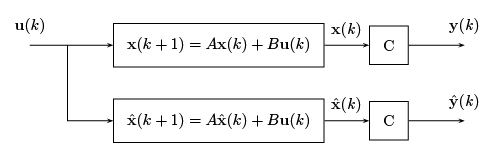
Figure 1: Open Loop Observer
The dynamics of this estimator are described by the following
where  is the estimate of x and
  is the estimate of y.
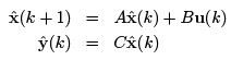
Let = − x be the estimation error.
Then the error dynamics are defined by
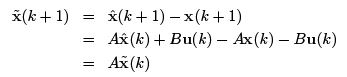
with the initial estimation error as
If the eigenvalues of A are inside the unit circle then will converge to 0. But we have no control over the convergence rate.
Moreover, A may have eigenvalues outside the unit circle. In that case will diverge from 0. Thus the open loop estimator is impractical.
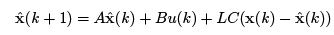
2.2 Luenberger State Observer
Consider the system x(k + 1) = Ax(k) + B u(k). Luenberger observer is shown in Figure 2. The observer dynamics can be expressed as:
 (1)
(1)
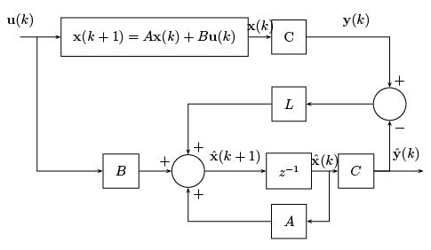
Figure 2: Luenberger observer
The closed loop error dynamics can be derived as:
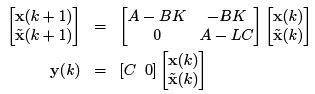
It can be seen that x˜ → 0 if L can be designed such that (A − LC ) has eigenvalues inside the unit circle of z -plane.
The convergence rate can also be controlled by properly choosing the closed loop eigenvalues.
Computation of Observer gain matrix L
The task is to place the poles of |A − LC |. Necessary and sufficient condition for arbitrary pole placement is that the pair should be controllable.
Assumption: The pair (A, C ) is observable. Thus, from the theorem of duality, the pair (AT , C T ) is controllable.
You should note that the eigenvalues of AT − CT LT are same as that of A − LC . It is same as a hypothetical pole placement problem for the system , using a control law
Example:
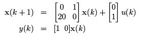
The observability matrix
is non singular. Thus the pair (A, C ) is observable. The observer dynamics are
L should be designed such that the observer poles are at 0.2 and 0.3.
We design LT such that AT − CT LT has eigenvalues at 0.2 and 0.3.

Using Ackermann’s formula, LT = [−0.5 20.06]. Thus

2.3 Controller with Observer
The observer dynamics:
 .
.
Combining with the system dynamics
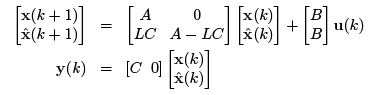
Since the states are unavailable for measurements, the control input is
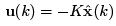
Putting the control law in the augmented equation
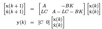
The error dynamics is
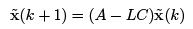
If we augment the above with the system dynamics, we get
where the dimension of the augmented system matrix is R2n×2n. Looking at the matrix one can easily understand that 2n eigenvalues of the augmented matrix are equal to the individual eigenvalues of A − BK and A − LC .
Conclusion: We can reach to a conclusion from the above fact is the design of control law, i.e., A − B K is separated from the design of the observer, i.e., A − LC .
The above conclusion is commonly referred to as separation principle.
The block diagram of controller with observer is shown in Figure 3.
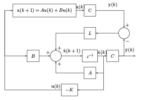
Figure 3: Controller with observer
FAQs on Lecture 34 - State Estimators or Observers - Electrical Engineering (EE)
| 1. What is a state estimator or observer? |  |
| 2. How does a state estimator work? | |
| 3. What are the applications of state estimators or observers? | |
| 4. What are the advantages of using state estimators or observers? | |
| 5. What are the limitations of state estimators or observers? | |


Top Courses for Electrical Engineering (EE)

Semester Notes
,Summary
,Extra Questions
,video lectures
,practice quizzes
,Viva Questions
,shortcuts and tricks
,Free
,Important questions
,study material
,MCQs
,Lecture 34 - State Estimators or Observers - Electrical Engineering (EE)
,ppt
,Lecture 34 - State Estimators or Observers - Electrical Engineering (EE)
,Previous Year Questions with Solutions
,Objective type Questions
,past year papers
,Lecture 34 - State Estimators or Observers - Electrical Engineering (EE)
,Exam
,mock tests for examination
,Sample Paper
;


Lecture 34 - State Estimators or Observers Free PDF Download
Importance of Lecture 34 - State Estimators or Observers
Lecture 34 - State Estimators or Observers Notes
Lecture 34 - State Estimators or Observers Electrical Engineering (EE) Questions
Study Lecture 34 - State Estimators or Observers on the App
|
© EduRev
|
Education Revolution
|


|


within 7 days!