Eigenvalues, Eigenvectors of Tensors - Civil Engineering (CE) PDF Download

Eigenvalues, eigenvectors of tensors
The scalar λi characterize eigenvalues (or principal values) of A if there exist corresponding nonzero normalized eigenvectors  (or principal directions or principal axes) of A, so that



To identify the eigenvectors of a tensor, we use subsequently a hat on the vector quantity concerned, for example,  .
Thus, a set of homogeneous algebraic equations for the unknown eigenvalues λ_i , i = 1,2,3, and the unknown eigenvectors  , i = 1,2,3, is
(A − λ_i1) = o, (i = 1,2,3; no summation).                                            (2.137)

For the above system to have a solution  ≠ o the determinant of the system must vanish. Thus,

det(A − λ_i1) = 0                                                                                        (2.138)

where



This requires that we solve a cubic equation in λ, usually written as



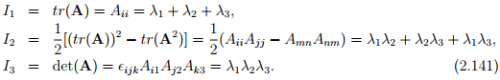
called the characteristic polynomial (or equation) for A, the solutions of which are the eigenvalues λ_i , i = 1,2,3. Here, I_i , i = 1,2,3, are the so-called principal scalar invariants of A and are given by



If A is invertible then we can compute I₂ using the expression I₂ = tr(A⁻¹ ) det(A). A repeated application of tensor A to equation (2.136) yields  i = 1,2,3, for any positive integer α. (If A is invertible then α can be any integer; not necessarily positive.) Using this relation and (2.140) multiplied by , we obtain the well-known Cayley-Hamilton equation:



It states that every second order tensor A satisfies its own characteristic equation. As a consequence of Cayley-Hamilton equation, we can express A^α in terms of A² , A, 1 and principal invariants for positive integer, α > 2. (If A is invertible, the above holds for any integer value of α positive or negative provided α ≠ {0, 1, 2}.)

For a symmetric tensor S the characteristic equation (2.140) always has three real solutions and the set of eigenvectors form a orthonormal basis {nˆi} (the proof of this statement is omitted). Hence, for a positive definite symmetric tensor A, all eigenvalues λi are (real and) positive since, using (2.136), we have λ_i = �  > 0, i = 1,2,3.

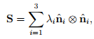
Any symmetric tensor S may be represented by its eigenvalues λ_i , i = 1,2,3, and the corresponding eigenvectors of S forming an orthonormal basis {}. Thus, S can be expressed as

                           (2.143)

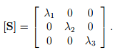
called the spectral representation (or spectral decomposition) of S. Thus, when orthonormal eigenvectors are used as the Cartesian basis to represent S then
                        (2.144)

The above holds when all the three eigenvalues are distinct. On the other hand, if there exists a pair of equal roots, i.e., λ₁ = λ₂ ≠  λ₃, with an unique eigenvector  associated with λ₃, we deduce that



where   and  denote projection tensors introduced in (2.109) and (2.110) respectively. Finally, if all the three eigenvalues are equal, i.e., λ₁ = λ₂ = λ₃ = λ, then

S = λ1,                                                                              (2.146)

where every direction is a principal direction and every set of mutually orthogonal basis denotes principal axes.
It is important to recognize that eigenvalues characterize the physical nature of the tensor and that they do not depend on the coordinates chosen.
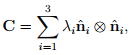
Square root theorem Let C be symmetric and positive definite tensor. Then there is a unique positive definite, symmetric tensor U such that

U² = C.                            (2.147)

We write  for U. If spectral representation of C is:

                         (2.148)


then the spectral representation for U is:

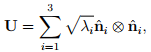                                           (2.149)

where we have assumed that the eigenvalues of C, λ_i are distinct. On the other hand if λ₁ = λ₂ = λ₃ = λ then

 (2.150)

If λ₁ = λ₂ = λ ≠ λ₃, with an unique eigenvector  associated with λ₃ then