Radiation - 2 - Electrical Engineering (EE) PDF Download

Radiation Zone Approximation
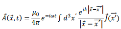
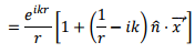
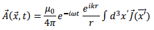
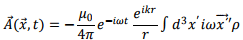
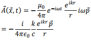
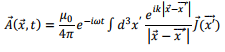
We had seen that the expression for the vector potential for a localized current distribution is given by
In near field approximation, this led to expression that was familiar to us in magnetostatics excepting for the time dependent multiplicative factor  leading to our describing the situation as “quasi-stationary”. We will not have much to say about the intermediate zone as this case is very complicated. However, the far field approximation or the radiation zone for which the distance of the point of observation from the source is much greater than both the typical source dimension and the wavelength of radiation is of great interest to us and will be described in the following.
Let us write  We expand
  and
and  as follows:
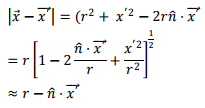
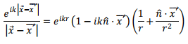
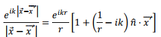
Thus
for situations where r<<x'.In a similar way, we have, keeping terms of the order of 1/r3 in Binomial expansion
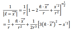
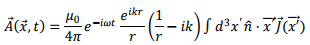
Using the above, we can write, retaining terms upto 
Electric Dipole Approximation
The lowest order approximation is to ignore the second term within bracket of the above. This gives
The integral above is rewritten by observing,
where we have used  and the fact that the time dependence is given by
  We replace each component of
  in the expression for vector potential by
  The integration over the first term is done by first converting it to a surface integral using the divergence theorem and letting the surface go toinfinity. Since the source dimension is confined to a limited region of space, this integral is zero and we are then left with,
The integral  is the electric dipole moment of the source. Hence, we can write,
where we have used 
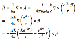
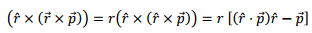
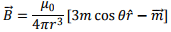
We can now obtain the expressions for the magnetic field and the electric field from the vector potential. Using the fact that  is a constant vector, we can write,
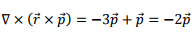
Thus the magnetic field direction is transverse to the direction of  We will see, however, that the electric field has a longitudinal component as well.
which gives
We have,
The first and the last terms of above are zero because  is a constant vector. We are left with
Substituting these, the electric field becomes

We reorganize the terms in the following fashion. Keep the first term within the first parenthesis in tact. For the second and the third terms, expand the vector triple product
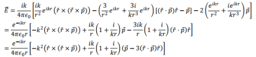
Note that, while the magnetic field was transverse, the electric field has a longitudinal component as well. Both these fields go as 1/r for large distances. However, for smaller distances, while the magnetic field vary as  the electric field goes as
  (the last term ).
In the radiation zone, we are only interested in large distance behaviour. In this regime, the field expressions are,
and the corresponding electric field is given by
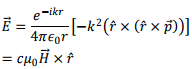
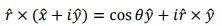
so that  and
and  are mutually perpendicular.
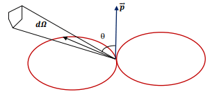
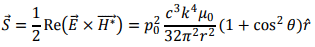
How does the emitted power, i.e., the average value of Poynting vector vary?
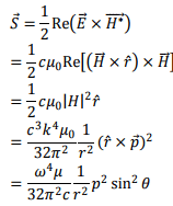
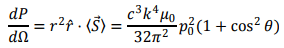
The amount of power flowing per unit solid anglein the direction of (θ, Ø) is given by
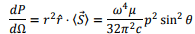
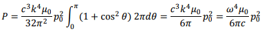
and the total radiated power is obtained by integrating over (θ, Ø). Since there is no azimuthal dependence, the integration over Ø gives 2π and we get,
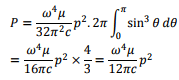
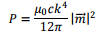
The following figure shows the “power pattern” in dipole approximation. It can be seen that the two lobes are symmetric about the dipole. The distance from the dipole to the lobe at any point gives the relative power in that direction with respect to the maximum. The total radiated power varies as the fourth power of the frequency.
Magnetic Dipole and Electric Quadrupole Approximation
We had started our discussion on radiation zone with the following expression for the vector potential,
Retaining terms up to order  we had approximated
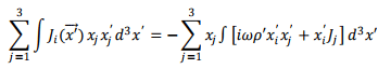
In the dipole approximation, we only retained the first term within the square bracket and ignored the remaining. Our next approximation is concerned with the second term. We will not write down the dipole term so that what we are discussing below is the correction to the dipole radiation. We consider
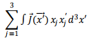
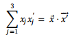
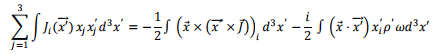
where we have taken out factors which are not concerned with the integration variable outside the integration.In order to perform the integration, let us write the dot product in an expanded form. Restricting only to the integration (the outside constants will be inserted later)
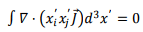
Using the argument given before, as the ettent of the source is limited, by extending the surface integral to infinite distances, we have, from the divergence theorem,
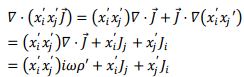
If we write this by expanding the divergence term, we have,
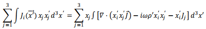
where, in the last step, we have used the equation of continuity. Inserting this into i-th component of the integral,
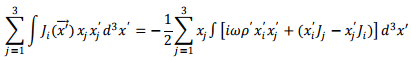
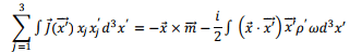
As mentioned before, the integral over the divergence is zero and we are left with
We replace the right hand side with half the term and add half of the left hand side to it
The term  is easily seen to be component of a cross product and can be written as
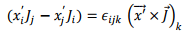
where  is the Levi-Civita symbol which is + 1 if i,j,k is an even permutation of 1,2 and 3, is −1 if it is an odd permutation and is zero if any pair of symols are equal. Using
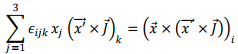
We also have,
Thus
Adding three components
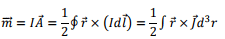
where the magnetic moment vector  is given by
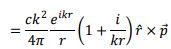
The term  is the magnetic dipole term and the remaining term is the electrical quadrupole term. Substituting these in the expression for the vector potential for the magnetic dipole term becomes,
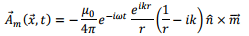
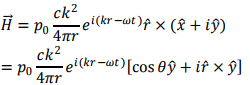
The magnetic field is now readily calculated. Suppressing the time variation,
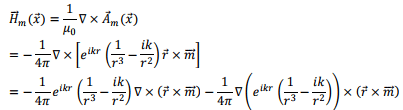
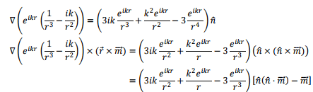
and
Combining these,
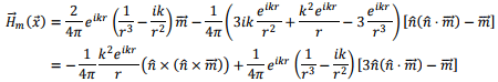
where we have restored the structure  for the central term of the second expression retaining the expanded form for the remaining.
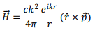
In the radiation zone, the first term, which varies as 1/r at large distances dominate and we have,
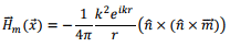
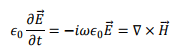
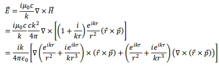
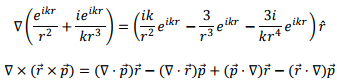
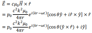
The corresponding electric field can be determined from Faraday’s law,
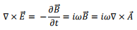
so that
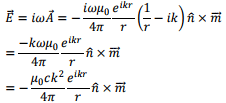
where we have retained only the leading term in radiation zone approximation.
The power radiated can be calculated in the same manner as we did for the electric dipole case,
[The above formulae were for two specific cases of radiating systems, viz. oscillating electric dipole and oscillating magnetic dipole. The power radiated from an arbitrary current and charge distribution is given by the formula

where the double dots indicate double differentiation with time. For the specific cases mentioned above, these boil down to respective formulae on taking the time average.
Tutorial Assignment
- A spherically symmetric charge distribution oscillates in a radial direction such that it remains spherically symmetric at all time. Show that no radiation is emitted.
- An electric dipole of strength 10−7 C-m oscillates at an angular frequency of 3 × 10⁸ rad/s. The dipole is placed along the z-axis. (a) Find the strength of the electric field measured by an observer located at (5,0,0) km. (b) What is the phase difference between the oscillation frequency of the dipole and that seen by this observer? (c) What is the average power measured at this location? (d) What would be the average power measured if the observer was located at (0,0,5) km instead of the position defined in (a)? (e) What is the total rate at which the dipole radiates power?
- A wire of length 1 m is bent in a circular loop to form a magnetic dipole antenna. The current in the dipole varies as |= |0 sin ωt with ω = 3 × 10⁸ rad/s and |0 = 2 A. Determine the electric and the magnetic field as seen by an observer at a large distance r from the dipole at an angle θto the axis of the loop. Calculate the total power radiated.
Solutions toTutorial Assignment
1. Spherical symmetry implies that both the electric and the magnetic field remains radial at all times. Using Gauss’s law, this implies 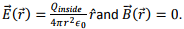 This implies the Poyntingvector
  hence there is no radiation.
2. Since the distance from the source is large, it is reasonable to assume that the observer is in the radiation zone. In this region we use 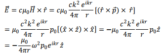
where we have used the fact that the observer is located along the x-axis .
(a) The field is thus directed opposite to the direction of the dipole moment vector, consi8stent with the fact that the dipole moment vector is along the direction from the negative to the positive charge. The strength of the electric field obtained by substituting given values is 0.18 V/m.
(b) As discussed in the last lecture, the wave generated at time t arrives at  at the observer’s location. Thus the phase difference between the wave at the source and that at the location of
  radians.
(c) Since the observer is in the equatorial plane θ= 90∘ . The power measured at this location is 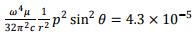 Watts.
(d) Along the axis of dipole θ= 0∘ so that no power is radiated in this direction.
(e) The total power radiated is given by 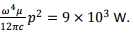
3. Take the dipole along the x-y plane with its axis being along the z-axis. Consider the position vector of the of observer to be in the x-z plane,
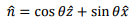
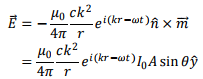
The magnetic moment vector is given by 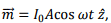 where A is the area of the loop. The complex magnetic field is given by
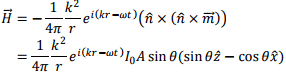
The electric field is given by
The average Poynting vector is given by
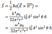
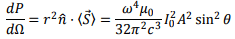
The power flowing out per unit solid angle is given by
The total power radiated is obtained by integrating over the solid angle and is given by
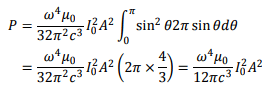
The area of the loop is obtained from its circumference of 1m to be  Substituting
  and other constants, we get the total power radiated to be 0.253 W.
Self Assessment Questions
1. Two point charges, q each, are attached to the ends of a rigid rod of length ℓ. The rod is rotated with an angular speed ω about an axis through the centre of the rod and perpendicular to it. Calculate the electric and the magnetic dipole moment of the system taking the centre of the rod as the origin. What is the total power radiated by this system?
2. An electric dipole of strength ρ0 initially lies along the x-axis centred at origin. The dipole rotates in the x-y plane about the z-axis at an angular frequency ω. Calculate the radiation field and the radiated power as seen by an observer in the x-z plane at an angle θ to the z-axis.
3. Neutron stars are a class of very dense stars consisting primarily of neutrons. The neutron star rotates with an angular frequency ω about an axis which makes an angle α with the direction of the magnetic moment. Assume the radius of the star to be 10 km and the angular frequency of rotation to be 100 rad/s about the z-axis which makes angle of α= 45∘ with the magnetic moment vector of the neutron star. Take the strength of the magnetic field at the magnetic equator to be 108T. Calculate the total power radiated.
Solutions to Self Assessment Questions
1. The electric dipole moment about the centre is zero as the position vector of the two (equal) charges are always directed oppositely. Magnetic dipole moment can be calculated by observing that charge 2q is rotating with a time period  which is equivalent to a current 4 πqω. The area of the current loop is
  Thus the magnetic moment is given by
 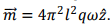 Both the electric and the magnetic dipoles are constant in time and hence there is no radiation emitted by the system.
2. The dipole vector can be written as

Since the observer is in x-z plane, y-direction is perpendicular to the direction of observation 
We can write  Note that
Using these, we can write the complex magnetic field as
The corresponding electric field is given by
The average Poynting vector is given by
The power flowing out per unit solid angle is given by
The total power radiated is given by integrating the above over the solid angle. Since there is no azimuthal dependence, we have,
3. The magnetic field of a dipole at  is given by the expression
where θ is the angle between and  At the equator, θ= 90∘ so that the strength of the magnetic field is

Substituting the given values, the magnitude of the magnetic field is 
As the star rotates about an axis which does not coincide with the magnetic moment vector, the direction of the magnetic moment vector precesses about the z-axis. This accounts for the radiation. It was pointed out that the magnetic dipole radiation power is proportional to the square of the second derivative of the magnetic moment. We can write
The magnetic moment vector as 
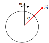

Substituting numerical values, one gets the power radiated to be 1.2 × 1029 W.
FAQs on Radiation - 2 - Electrical Engineering (EE)
| 1. What is radiation in the context of electrical engineering? |  |
| 2. How does radiation affect electronic devices? | |
| 3. What are the safety considerations for radiation exposure in electrical engineering? | |
| 4. How can radiation be controlled or mitigated in electrical engineering applications? | |
| 5. What are the potential health risks associated with radiation exposure in electrical engineering? | |


Radiation - 2 - Electrical Engineering (EE)
,practice quizzes
,Summary
,Important questions
,video lectures
,Extra Questions
,Viva Questions
,Sample Paper
,Semester Notes
,study material
,Previous Year Questions with Solutions
,ppt
,Objective type Questions
,Radiation - 2 - Electrical Engineering (EE)
,mock tests for examination
,Free
,Radiation - 2 - Electrical Engineering (EE)
,shortcuts and tricks
,past year papers
,Exam
,MCQs
;


Radiation - 2 Free PDF Download
Importance of Radiation - 2
Radiation - 2 Notes
Radiation - 2 Electrical Engineering (EE) Questions
Study Radiation - 2 on the App
|
© EduRev
|
Education Revolution
|


|


within 7 days!