Lecture 37 - Output Feedback Design Examples | 6 Months Preparation for GATE Electrical - Electrical Engineering (EE) PDF Download

Lecture 37 - Output feedback design examples, Control Systems
1 Output feedback design examples
In the last lecture, we have discussed about the incomplete state feedback design and output feedback design. In this lecture we would solve some examples to make the procedure properly understood.
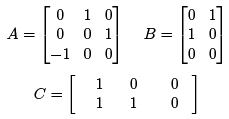
Example 1: Let us consider the following system
x(k + 1) = Ax(k) + Bu(k)
y(k) = C x(k)
for which the A, B , C matrices are as follows
We know, for output feedback,
u(k) = −Gy(k)
where the matrix G has to be designed. Since C has rank 2 and the rank of B is also 2, minimum 2 eigenvalues can be placed at desired locations. Let these two be 0.1 and 0.2. The characteristic equation of A is
|zI − A| = z3 + 1
B ∗ is written as
B∗ = BW =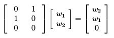
which has two independent parameters in terms of w1 and w2. Controllability matrix for the pair (A, B ∗) is
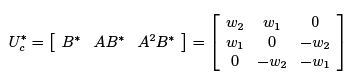
It will be non singular if 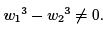 Let
Let
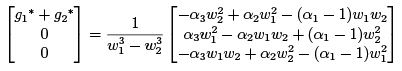
G∗ =[g1∗ g2∗]C
Then
Since C has a rank of 2, G∗C has two independent parameters in terms of g1∗ and g2∗. The closed loop characteristic equation is
φ(z) = z3 + α3z2 + α2z + α1 = 0
Thus
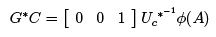
G∗C =[ 0 0 1 ] Uc∗−1 φ(A)
or,
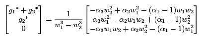
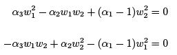
The last row in the above equation corresponds to the following constraint equation.
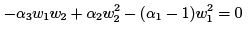 (1)
(1)
Since 2 of the three eigenvalues can be arbitrarily placed, w1 and w2 can be arbitrary provided the condition  is satisfied. But they should be selected such that the third eigenvalue is stable. This puts an additional constraint on w1 and w2.
For example, the necessary condition for the closed loop system to be stable is |α| < 1.
To satisfy this condition, w2 cannot be equal to zero.
For z = 0.1 and 0.2 to be the roots of the characteristic equation
z3 + α3z2 + α2z + α1 = 0
the following equations must be satisfied
α1 + 0.001 + α30.01 + 0.1α2 = 0
α1 + 0.008 + α30.04 + 0.2α2 = 0
Simplifying the above equations,
α2 + 0.3α3 + 0.07 = 0 (2) α1 − 0.02α3 − 0.006 = 0 (3)
Solving equations (1), (2) and (3) together
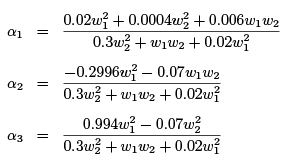
If we set w1 = 0 and w2 = 1, we get α1 = 0.00133, α2 = 0 and α3 = −0.23333.
With the above coefficients we find the roots to be z1 = 0.1, z2 = 0.2 and z3 = −0.0667.
Thus the third pole is placed within the unit circle and the closed loop system is stable.
There also exist some other combinations of w1 and w2 for which z1 = 0.1, z2 = 0.2 and the closed loop system is stable.
Putting the values of w1 and w2 and corresponding α1, α2 and α3 in the expression of G∗C , we get
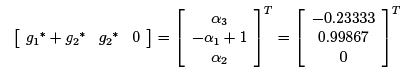
Thus the feedback matrix can be calculated as
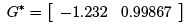
Hence,

Example 2: Consider the same system as in the previous example except for the fact that now
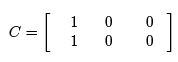
which has rank 1. This implies that
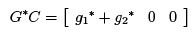
which has only one independent parameter in terms of g1∗ and g2∗. Thus
Last two rows of the above equation are constrained to be zero. Thus we can only assign w1 or w2 arbitrarily, not both. The constraint equations are as follows.
If we want two closed loop eigenvalues to be placed at z = 0.1 and z = 0.2, we will altogether have four equations with five unknowns. Only one of these five unknowns can be assigned arbitrarily.
But these four equations would be nonlinear in w1 and w2, hence difficult to solve. The simpler way would be to use the following equation

Only two coefficients can be arbitrarily assigned. Since the constant term is equal to 1, the system cannot be stabilized with output feedback.
|
675 videos|1379 docs|882 tests
|
FAQs on Lecture 37 - Output Feedback Design Examples - 6 Months Preparation for GATE Electrical - Electrical Engineering (EE)
| 1. What is output feedback design in control systems? |  |
| 2. Why is output feedback design important in control systems? | |
| 3. What are the advantages of using output feedback design? | |
| 4. What are the limitations of output feedback design? | |
| 5. How is output feedback design implemented in practice? | |


Objective type Questions
,Extra Questions
,Lecture 37 - Output Feedback Design Examples | 6 Months Preparation for GATE Electrical - Electrical Engineering (EE)
,past year papers
,Lecture 37 - Output Feedback Design Examples | 6 Months Preparation for GATE Electrical - Electrical Engineering (EE)
,Important questions
,video lectures
,Sample Paper
,shortcuts and tricks
,Lecture 37 - Output Feedback Design Examples | 6 Months Preparation for GATE Electrical - Electrical Engineering (EE)
,Summary
,practice quizzes
,Viva Questions
,study material
,Previous Year Questions with Solutions
,ppt
,Exam
,Semester Notes
,mock tests for examination
,MCQs
,Free
;


Lecture 37 - Output Feedback Design Examples Free PDF Download
Importance of Lecture 37 - Output Feedback Design Examples
Lecture 37 - Output Feedback Design Examples Notes
Lecture 37 - Output Feedback Design Examples Electrical Engineering (EE) Questions
Study Lecture 37 - Output Feedback Design Examples on the App
|
© EduRev
|
Education Revolution
|


|


