Lecture 33 - Introduction to Optimal Control - Electrical Engineering (EE) PDF Download

Lecture 38 - Introduction to optimal control, Control Systems
1 Introduction to optimal control
In the past lectures, although we have designed controllers based on some criteria, but we have never considered optimality of the controller with respect to some index. In this context, Linear Quadratic Regular is a very popular design technique.
The optimal control theory relies on design techniques that maximize or minimize a given performance index which is a measure of the effectiveness of the controller.
Euler-Lagrange equation is a very popular equation in the context of minimization or maximization of a functional.
A functional is a mapping or transformation that depends on one or more functions and the values of the functionals are numbers. Examples of functionals are performance indices which will be introduced later.
In the following section we would discuss the Euler-Lagrange equation for discrete time systems.
1.1 Discrete Euler-Lagrange Equation
A large class of optimal digital controller design aims to minimize or maximize a performance index of the following form.
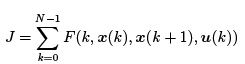
where F (k, x(k), x(k + 1), u(k)) is a differentiable scalar function and x(k) ∈ Rn, u(k) ∈ Rm.
The minimization or maximization of J is sub ject to the following constraint.
x(k + 1) = f (k, x(k), u(k))
The above can be the state equation of the system, as well as other equality or inequality constraints.
Design techniques for optimal control theory mostly rely on the calculus of variation, according to which, the problem of minimizing one function while it is sub ject to equality constraints is solved by adjoining the constraint to the function to be minimized.
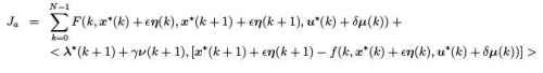
Let λ(k + 1) ∈ Rn×1 be defined as the Lagrange multiplier. Adjoining J with the constraint equation,
 F (k, x(k), x(k + 1), u(k))+ < λ(k + 1), [x(k + 1) − f (k, x(k), u(k))] >
where < . > denotes the inner product.
Calculus of variation says that the minimization of J with constraint is equivalent to the minimization of Ja without any constraint.
Let x∗(k), x∗(k + 1), u∗(k)) and λ∗(k + 1) represent the vectors corresponding to optimal tra jectories. Thus one can write
x(k) = x∗(k) + ∈η(k)
x(k + 1) = x∗(k + 1) + ∈η(k + 1)
u(k) = u∗(k) + δµ(k)
λ(k + 1) = λ∗(k + 1) + γ ν (k + 1)
where η(k), µ(k), ν (k) are arbitrary vectors and ∈, δ, γ are small constants.
Substituting the above four equations in the expression of Ja,
To simplify the notation, let us denote Ja as
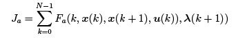
Expanding Fa using Taylor series around x∗(k), x∗(k + 1), u∗(k)) and λ∗(k + 1),
we get Fa(k, x(k), x(k + 1), u(k), λ(k + 1)) = Fa(k, x∗(k), x∗(k + 1), u∗(k), λ∗(k + 1)) +
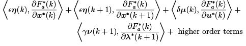
where

The necessary condition for Ja to be minimum is
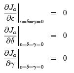
Substituting Fa into the expression of Ja and applying the necessary conditions,
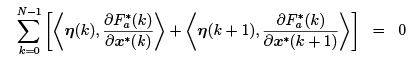 (1)
(1)
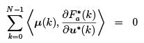 (2)
(2)
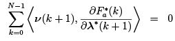 (3)
(3)
Equation (1) can be rewritten as
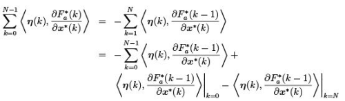
where

Rearranging terms in the last equation, we get
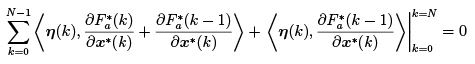
According to the fundamental lemma of calculus of variation, equation (4) is satisfied for any η(k) only when the two components of the equation are individually zero. Thus,
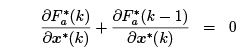 (5)
(5)
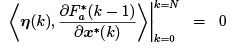 (6)
(6)
Equation (5) is known as the discrete Euler-Lagrange equation and equation (6) is called the transversality condition which is nothing but the boundary condition needed to solve equation (5).
Discrete Euler-Lagrange equation is the necessary condition that must be satisfied for Ja to be an extremal.
With reference to the additional conditions (2) and (3), for arbitrary µ(k) and ν (k + 1),
 = 0, j = 1, 2, · · · m (7)
 0, i = 1, 2, · · · n (8)
Equation (8) leads to
x ∗(k + 1) = f (k, x∗(k), u∗(k))
which means that the state equation should satisfy the optimal tra jectory. Equation (7) gives the optimal control u∗(k) in terms of λ∗(k + 1)
In a variety of the design problems, the initial state x(0) is given. Thus η(0) = 0 since x(0) is fixed. Hence the tranversality condition reduces to
Again, a number of optimal control problems are classified according to the final conditions.
If x(N ) is given and fixed, the problem is known as fixed-endpoint design. On the other hand, if x(N ) is free, the problem is called a free endpoint design.
For fixed endpoint (x(N ) = fixed, η(N ) = 0) problems, no transversality condition is required to solve.
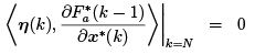
For free endpoint the transversality condition is given as follows.
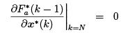 .
.
For more details, one can consult Digital Control Systems by B. C. Kuo.
FAQs on Lecture 33 - Introduction to Optimal Control - Electrical Engineering (EE)
| 1. What is optimal control? |  |
| 2. How is optimal control different from traditional control? | |
| 3. What are the key components of an optimal control problem? | |
| 4. What are some common techniques used in solving optimal control problems? | |
| 5. What are some applications of optimal control? | |


Top Courses for Electrical Engineering (EE)

practice quizzes
,Semester Notes
,past year papers
,study material
,Lecture 33 - Introduction to Optimal Control - Electrical Engineering (EE)
,shortcuts and tricks
,ppt
,Lecture 33 - Introduction to Optimal Control - Electrical Engineering (EE)
,Sample Paper
,mock tests for examination
,Important questions
,Viva Questions
,Free
,MCQs
,Previous Year Questions with Solutions
,Lecture 33 - Introduction to Optimal Control - Electrical Engineering (EE)
,video lectures
,Summary
,Exam
,Extra Questions
,Objective type Questions
;


Lecture 33 - Introduction to Optimal Control Free PDF Download
Importance of Lecture 33 - Introduction to Optimal Control
Lecture 33 - Introduction to Optimal Control Notes
Lecture 33 - Introduction to Optimal Control Electrical Engineering (EE) Questions
Study Lecture 33 - Introduction to Optimal Control on the App
|
© EduRev
|
Education Revolution
|


|


within 7 days!