Lecture 40 - Linear Quadratic Regulator - Electrical Engineering (EE) PDF Download

Lecture 40 - Linear Quadratic Regulator, Control Systems
1 Linear Quadratic Regulator
Consider a linear system modeled by
x(k + 1) = Ax(k) + Bu(k), x(k0) = x0
where x(k) ∈ Rn and u(k) ∈ Rm. The pair (A, B ) is controllable.
The ob jective is to design a stabilizing linear state feedback controller u(k) = −Kx(k) which will minimize the quadratic performance index, given by,
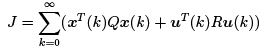
where, Q = QT ≥ 0 and R = RT > 0. Such a controller is denoted by u∗.
We first assume that a linear state feedback optimal controller exists such that the closed loop system
x(k + 1) = (A − BK )x(k)
is asymptotically stable.
This assumption implies that there exists a Lyapunov function V (x(k)) = x(k)T P x(k) for the closed loop system, for which the forward difference
∆V (x(k)) = V (x(k + 1)) − V (x(k))
is negative definite.
We will now use the theorem as discussed in the previous lecture which says if the controller u∗ is optimal, then

If we substitute ∆V in the above expression, we get

Taking derivative of the above function with respect to u(k),
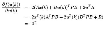
The matrix BTPB + R is positive definite since R is positive definite, thus it is invertible.
Hence,
u∗(k) = −(BT P B + R)−1BT P Ax(k) = −K x(k)
where K = (BT P B + R)−1BT P A. Let us denote BT P B + R by S . Thus
u∗(k) = −S −1BT P Ax(k)
We will now check whether or not u∗ satisfies the second order sufficient condition for minimization. Since
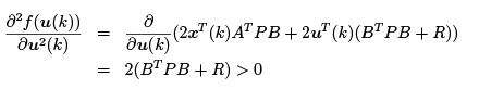
u ∗satisfies the second order sufficient condition to minimize f .
The optimal controller can thus be constructed if an appropriate Lyapunov matrix P is found.
For that let us first find the closed loop system after introduction of the optimal controller. x(k + 1) = (A − BS −1BT P A)x(k)
Since the controller satisfies the hypothesis of the theorem, discussed in the previous lecture,
x T(k + 1)P x(k + 1) − xT (k)P x(k) + xT (k)Qx(k) + u∗T (k)Ru∗(k) = 0
Putting the expression of u∗ in the above equation,
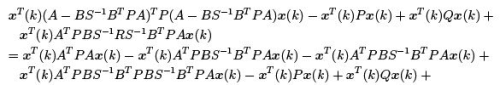
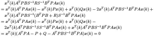
The above equation should hold for any value of x(k). Thus
which is the well known discrete Algebraic Riccati Equation (ARE). By solving this equation we can get P to form the optimal regulator to minimize a given quadratic performance index.
Example 1: Consider the following linear system
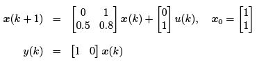
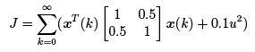
Design an optimal controller to minimize the following performance index.
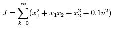
Also, find the optimal cost.
Solution: The performance index J can be rewritten as
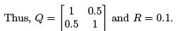
Let us take P as
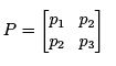
Then,
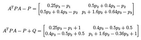
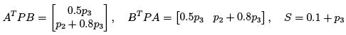
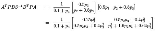
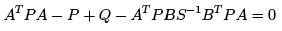
The discrete ARE is
ATPA−P+Q − ATPBS−1BTPA = 0
Or,
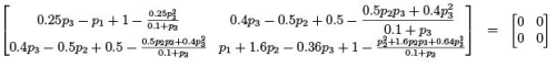
We can get three equations from the discrete ARE. These are
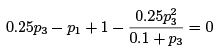
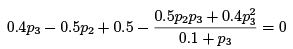

Since the above three equations comprises three unknown parameters, these parameters can be solved uniquely, as
p1 = 1.0238, p2 = 0.5513, p3 = 1.9811
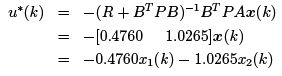
The optimal control law can be found out as
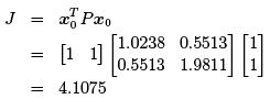
The optimal cost can be found as
FAQs on Lecture 40 - Linear Quadratic Regulator - Electrical Engineering (EE)
| 1. What is a linear quadratic regulator? |  |
| 2. How does a linear quadratic regulator work? | |
| 3. What are the advantages of using a linear quadratic regulator? | |
| 4. Can a linear quadratic regulator be used for nonlinear systems? | |
| 5. How is the performance of a linear quadratic regulator evaluated? | |


Top Courses for Electrical Engineering (EE)

study material
,Semester Notes
,Sample Paper
,past year papers
,Viva Questions
,ppt
,video lectures
,Free
,Lecture 40 - Linear Quadratic Regulator - Electrical Engineering (EE)
,Objective type Questions
,Extra Questions
,Exam
,practice quizzes
,Lecture 40 - Linear Quadratic Regulator - Electrical Engineering (EE)
,mock tests for examination
,Summary
,Lecture 40 - Linear Quadratic Regulator - Electrical Engineering (EE)
,Important questions
,Previous Year Questions with Solutions
,MCQs
,shortcuts and tricks
;


Lecture 40 - Linear Quadratic Regulator Free PDF Download
Importance of Lecture 40 - Linear Quadratic Regulator
Lecture 40 - Linear Quadratic Regulator Notes
Lecture 40 - Linear Quadratic Regulator Electrical Engineering (EE) Questions
Study Lecture 40 - Linear Quadratic Regulator on the App
|
© EduRev
|
Education Revolution
|


|


