Solutions to Laplace’s Equations - 3 - Electronics and Communication Engineering (ECE) PDF Download

Laplace’s Equation in Spherical Coordinates :
We continue with our discussion of solutions of Laplace’s equation in spherical coordinates by giving some more examples.
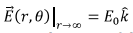
Example 3 : A conducting sphere in a uniform electric field This is a classic problem. Let the sphere be placed in a uniform electric field in z direction  Though we expect the field near the conductor to be modified, at large distances from the conductor, the field should be uniform and we have,
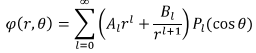
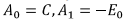
Clearly, we have azimuthal symmetry because of the sphere but the direction of the electric field will bring in polar angle dependence. As a result, the potential at large distances has the following form :

where C is a constant. The conductor being a equipotential, the field lines strike its surface normally.
The lines of force near the sphere look as follows :
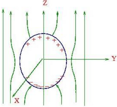
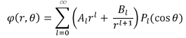
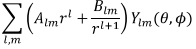
As shown here, there will be charges induced on the surface. On the surface, the potential is constant (it is a conductor) φ0. Since there are no sources, outside the sphere, the potential satisfies the Laplace’s equation. As there is azimuthal symmetry in the problem, the potential is given by,
Note that the potential expression cannot contain l = 0 term in the second term because a potential  implies a delta function source.
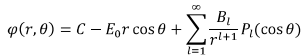
At large distances from the conductor, the above expression must match with 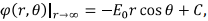 which we had obtained earlier. As all terms containing Bl vanish at large distances, we need to compare with the terms containing
  are the only non-zero terms,
Thus,
We will now use the boundary condition on the surface of the conductor, which is a constant, say φ0 This implies
Comparing both sides, we have, 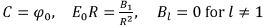
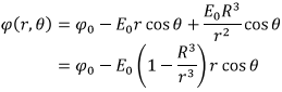
The potential outside the sphere is thus given by,
The electric field is given by the negative gradient of the potential,
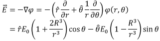
The charge density on the sphere is given by the normal component (i.e. radial component) of the electric field on the surface (r=R) and is given by
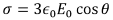
The charge induced on the upper hemisphere is (recall that θ is measured from the north pole of the sphere as z direction points that way,
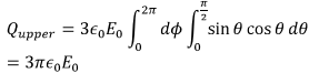
The charge on the lower hemisphere is  so that the total charge is zero, as expected.
Note that an uncharged sphere in an electric field modifies the potential by  You may recall that the potential due to a dipole placed at the origin is
Thus the sphere behaves like a dipole of dipole moment 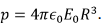
If the sphere had a charge Q, it would modify the potential by an additional Coulomb term.
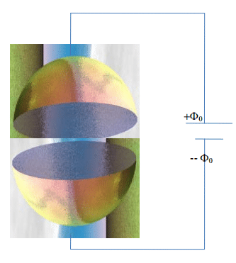
Example 4 : Conducting hemispherical shells joined at the equator :
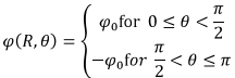
Consider two conducting hemispherical shells which are joined at the equator with negligible separation between them. The upper hemisphere is mained at a potential of  while the lower is maintained at
  .We are required to find the potential within the sphere.
Since the system gas azimuthal symmetry, we can expand the potential in terms of Legendre polynomials,
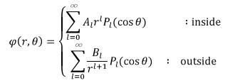
Using the argument we have given earlier, the relevant equation for the potential inside and outside the sphere are as follows :
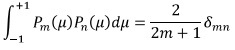
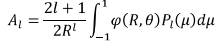
We will determine a few of the coefficients in these expansions. To find the coefficients, we use the orthogonality property of the Legendre polynomials,
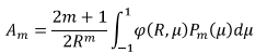
Using this we have,
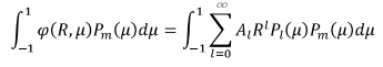
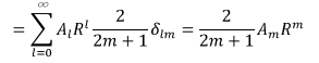
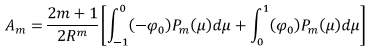
Thus,
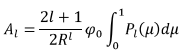
Since the potential is constant in two hemispheres, we split this integral from  corresponding to
 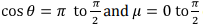 corresponding to
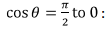
We know that  is a polynomial in μ, containing only odd powers of μ if m is off and only even powers of μ if m is even, the degree of polynomial being m. It can be easily seen that for even values of m, the above integral vanishes and only m that give non zero value are those which are odd. We will calculate a few such coefficients.
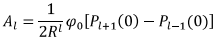
Take m=1 for which  the integrals within the square bracket adds up to φ0, so that we get
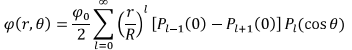
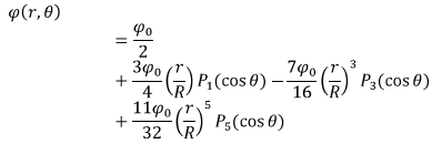
Take m=3 for which 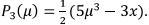 The integrals add up to
  so that we get
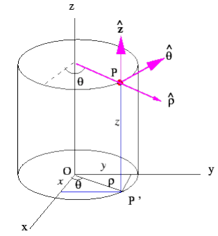
Laplace’s Equation in Cylindrical Coordinates :
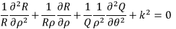
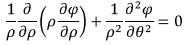
In cylindrical coordinates , Laplace’s equation has the following form :
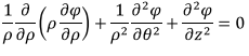
As before, we will attempt a separation of variables, by writing,
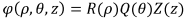
Substituting this into Laplace’s equation and dividing both sides of the equation by 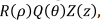 we get,
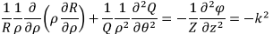
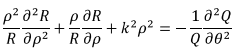
where, as before, we have used the fact that the first two terms depend on p and θ while the third term depends on z alone. Here -k2 is a constant and we have not yet specified its nature. We can easily solve the z equation,
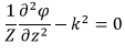
which has the solution,

(Remember that we have not specified k, if it turns out to be imaginary, our solution would be sine and cosine functions. In the following discussion we choose the hyperbolic form.)
Let us now look at the equation for R and Q, Expanding the first term,
Multiplying throughout by p2, we rewrite this equation as
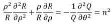
Once again, we notice that the left hand side depends only on ρ while the right hand side depends on θ only. Thus we must have,
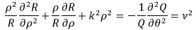
where v2 is an yet unspecified constant. The angle equation can be easily solved,
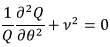
which has the solution

The domain of θ is [0:2π]. Since the potential must be single valued, 
 which requires ν must be an integer.
The radial equation now reads
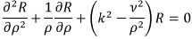
The above can be written in a compact form by defining  in terms of which the equation reads,
This equation is known as the Bessel equation and its solutions are known as Bessel Functions. We will not solve this equation but will point out the nature of its solutions. Being a second order equation, there are two independent solutions, known as Bessel functions of the first and the second kind. The first kind is usually referred to as Bessel functions whereas the second kind is also known as Neumann functions.
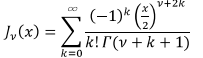
The Bessel functions of order ν is given by the power series,
Some of the limiting values of the function are as follows:
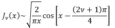
For 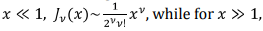 the function oscillates and has the form
When ν is an integer, 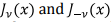 are not independent and are related by
 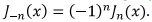 The variation of the Bessel function of some of the integral orders are given in the following figure.
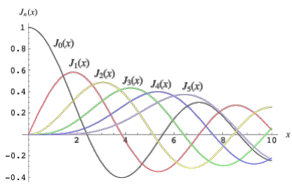
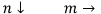
It can be seen that other that the zeroth order Bessel function, all Bessel functions vanish at the origin. In addition the Bessel functions have zeros at different values of their argument. The following table lists the zeros of Bessel functions. In the following knm denotes the m-th zero of Bessel function of order n.
 | 1 | 2 | 3 | |
| k0m | 0 | 2.406 | 5.520 | 8.654 |
| k1m | 1 | 3.832 | 7.016 | 10.173 |
| k2m | 2 | 5.136 | 8.417 | 11.620 |
Higher roots are approximately located at 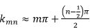
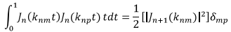
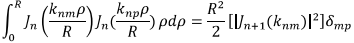
Bessel functions satisfy orthogonality condition,
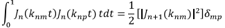
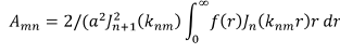
Another usefulness of Bessel function lies in the fact that a piecewise continuous function f defined in [0,a] with f(a)=0 can be expanded as follows :
Using orthogonality property of Bessel functions, we get,
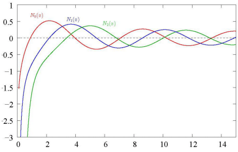
The second kind of Bessel function, viz., the Neumann function, diverges at the origin and oscillates for larger values of its argument ,
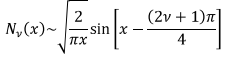

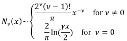
where  Like the Bessel function of the first kind, the Neumann functions are also not independent for integral values of n
 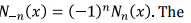 variation of the Neumann function are as shown below.
The solution of the radial equation can be written as
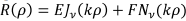
(If in the solution of z equation we had chosen k to be imaginary, the argument of the Bessel functions would be imaginary)
The complete solution is obtained by summing over all values of k and ν.
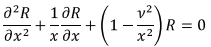
Special Case : A system with potential independent of z: In problems such as a long conductor, the symmetry of the problem makes the potential independent of z coordinates. In such cases, the problem is essentially two dimensional, the Laplace’s equation being,
A separation of variables of the form 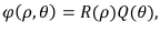 gives us, on expanding the first term,
The solution for Q(θ), is given by

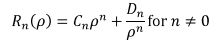
where, as before, singlevaluedness of the potential requires that n is an integer. The radial equation,
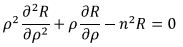
has a solution
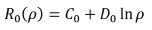
And for n=0
Example : An uncharged cylinder in a uniform electric field.
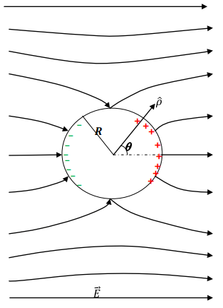
Like the problem of sphere in an electric field, we will discuss how potential function for a uniform electric field is modified in the presence of a cylinder. Let us take the electric field directed along the x-axis and we further assume that the potential does not have any z dependence.
As before, at large distances, the potential is that corresponding to a constant electric field in the x direction, i.e 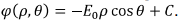 The charges induced on the conductor surface produce their own potential which superpose with this potential to satisfy the boundary condition on the surface of the conductor. Since there is no z dependence, the general solution of the Laplace’s equation, as explained above is,
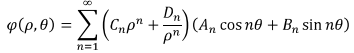
Here we have not taken n=0 term because its behavior is logarithmic which diverges at infinite distances. At large distances, the asymptotic behavior of this should match with the potential corresponding to the uniform field. Thus we choose the term proportional to 
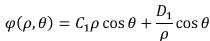
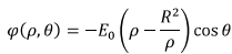
Clearly  We need to determine the constant D1. If the potential on the surface of the cylinder is taken to be zero, we must have for all angles θ,
  Substituting these, we get,
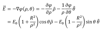
The electric field is given by the gradient of the potential, and is
The charge density on the surface of the conductor is the normal component of the electric field multiplied with 

Like in the case of the sphere, you can check that the total charge density is zero.
Tutorial Assignment
1. A cylindrical shell of radius R and length L has its top cap maintained at a constant potential φ0, its bottom cap and the curved surface are grounded. Obtain an expression for the potential within the cylinder.
2. A unit disk  has no sources of charge on it. The potential on the rim
  is given by 2 sin 4θ, where θ is the polar angle. Obtain an expression for potential inside the disk.
3. Consider two hemispherical shells of radius R where the bottom half is kept at zero potential and the top half is maintained at a constant potential φ0, Obtain an expression for the potential inside the shell.
Solutions to Tutorial Assignment
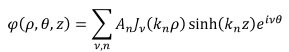
1. Take the bottom cap in the x-y plane with its centre at the origin and the z axis along the axis of the cylinder. Since the potential at z=0 is zero, we take 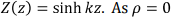 is within the cylinder, Neumann functions are excluded from the solution and we have,
Since the potential on the curved surface is zero irrespective of the azimuthal angle, we must v = 0. This gives,
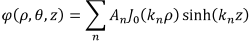
The potential at  also vanishes, giving
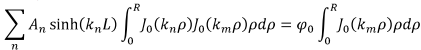
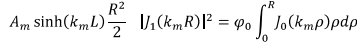
  This determines the values of kn being given by the zeros of Bessel function of order zero. Finally, the boundary condition on the top cap,
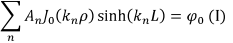
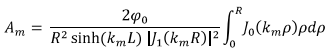
The coefficients An are determined by the orthogonal property of Bessel functions,
using which we have, substituting 
Multiply both sides of eqn. (I) with 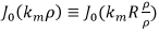 and integrate from 0 t0 R,
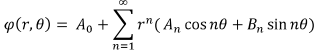
2. Laplace’s equation in polar coordinates is 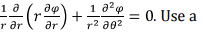 separation of variables
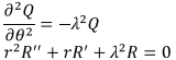
which have the solution  Here we have used the singlevaluedness of the potential to conclude that λ is an integer. The solution of the radial equation is
  The constant D must be zero because the function must be well behaved at the origin. Likewise the solution of the radial equation for n=0 is a logarithmic function the coefficient of which also vanishes for the same reason. Thus the solution is of the form,
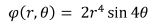
We can determine the coefficients by the boundary condition given at r=1,
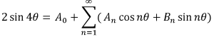
Clearly,  all coefficients other than B4 are also zero and B4 = 2.
3. See example 4 of lecture notes. Inside the sphere the potential is given by
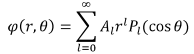
Using the orthogonality property of the Legendre polynomial,
where,  Using the fact that only one half of the sphere is maintained at constant potential while the other half is at zero potential, we have,
The integral can be looked up from standard tables,
Thus,
Using standard table for Legendre polynomials we have,
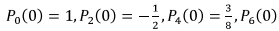
 etc. while all odd orders are zero. Thus,
Self Assessment Quiz
1. A conducting sphere of radius R is kept in an electrostatic field given by  Obtain an expression for the potential in the region outside the sphere and obtain the charge density on the sphere
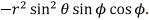
2. A unit disk  has no sources of charge on it. The electric field on the rim
  is given by
 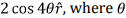 is the polar angle. Obtain an expression for potential inside the disk.
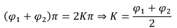
3. (Hard Problem) A cylindrical conductor of infinite length has its curved surfaces divided into two equal halves, the part with polar angle  has a constant potential φ1 while the remaining half is at a potential φ2.Obtain an expression for the potential inside the cylinder. Verify your result by calculating the potential on the surface at
  and at
Solutions to Self Assessment Quiz
1. The potential corresponding to the electric field is 
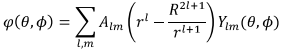
 Using the table for Spherical harmonics, the potential can be expressed as
 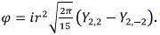 The general expression for solution of Laplace’s equation is
The boundary conditions to be satisfied are
(i) For all 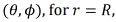 the potential is constant, which we take to be zero. This implies
 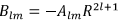 for all m. This makes the potential expression to be
(ii) For large distances, 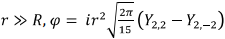 in this limit,, the second term for the expression for potential goes to zero and we are left with,
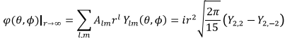
Comparing, we get only non-zero value of to be 2 and the corresponding m values as +2. Thus, the potential has the form
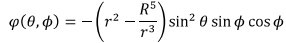
The surface charge density is given by
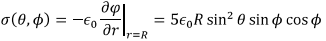
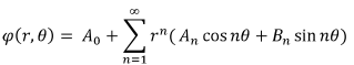
2. The solution of Laplace’s equation on a unit disk is given by (see tutorial problem)
The electric field is given by the negative gradient of potential. Since the field is given to be radial,
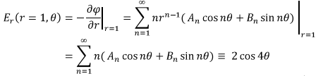
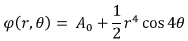
This gives all coefficients other than B4 to be zero and  The coefficient A0, however remains undetermined.
3. Because of symmetry along the z axis, the potential can only depend on the polar coordinates (p, θ) . By using a separation of variables, we can show, as shown in the lecture, the angular part Q(θ) = 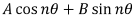 The radial equation has the solution
  we have ignored n=0 solution because it gives rise to logarithm in radial coordinate which diverges at origin. Thus the general solution for the potential is
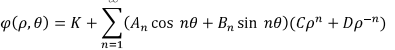
where K is a constant. Further, the constant D must be zero otherwise the potential would diverge at p = 0. Let us now apply the boundary conditions, For p = R,
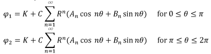
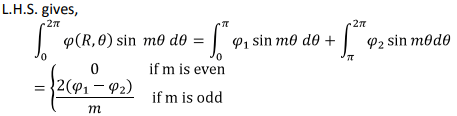
Integrate the first expression from  and the second expression from
  and add. The integration over the second term on the right hand side of the two expressions is equal to an integration from 0 to 2π and the integral vanishes. We are left with
Thus the potential expression at p = R becomes

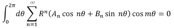
To evaluate the coefficients An, multiply both sides by cos mθ and integrate from 0 to 2π,
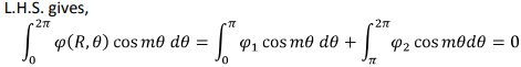
Similarly, the first term on the right also gives zero.
We are left with
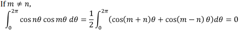
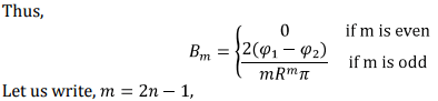
These integrals can be done by elementary methods,
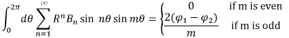
To determine the coefficients Bn, multiply both sides of (I) by sin mθ and integrate from 0 to 2π,
The first term on the right gives zero.
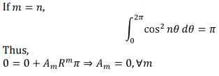
We are left with
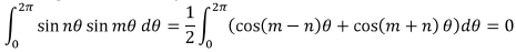
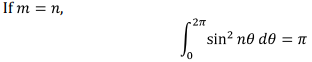
The integral can be easily done If m ≠ n,
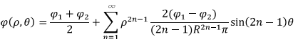
We have the final expression for the potential,
To verify that this is consistent with the given boundary conditions, let us evaluate the potential at 
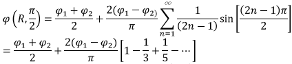
The infinite series has a value 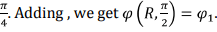 Similarly, one can check that
FAQs on Solutions to Laplace’s Equations - 3 - Electronics and Communication Engineering (ECE)
| 1. What is Laplace's equation and why is it important in electronics and communication engineering? |  |
| 2. How can Laplace's equation be solved? | |
| 3. What are the applications of Laplace's equation in electronics and communication engineering? | |
| 4. Can Laplace's equation be used to solve time-varying problems in electronics and communication engineering? | |
| 5. Are there any limitations or assumptions associated with Laplace's equation in electronics and communication engineering? | |


Top Courses for Electronics and Communication Engineering (ECE)
Exam
,Summary
,mock tests for examination
,practice quizzes
,video lectures
,Previous Year Questions with Solutions
,Extra Questions
,Free
,study material
,past year papers
,MCQs
,Objective type Questions
,Solutions to Laplace’s Equations - 3 - Electronics and Communication Engineering (ECE)
,Sample Paper
,Solutions to Laplace’s Equations - 3 - Electronics and Communication Engineering (ECE)
,Viva Questions
,Solutions to Laplace’s Equations - 3 - Electronics and Communication Engineering (ECE)
,ppt
,shortcuts and tricks
,Important questions
,Semester Notes
;


Solutions to Laplace’s Equations - 3 Free PDF Download
Importance of Solutions to Laplace’s Equations - 3
Solutions to Laplace’s Equations - 3 Notes
Solutions to Laplace’s Equations - 3 Electronics and Communication Engineering (ECE) Questions
Study Solutions to Laplace’s Equations - 3 on the App
|
© EduRev
|
Education Revolution
|


|


