Normal and shear strain
From now on we shall in this course, study the response of bodies only for cases when the value of the components of both the Lagrangian and Eulerian displacement gradient are small. As we have shown above, this means that not only does the changes in length be small but the rotations also needs to be small. Under these severe but practically reasonable assumptions, the strain-displacement relation is
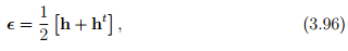
where we stop distinguishing between Lagrangian and Eulerian gradient, as they would be approximately the same. Thus, the Cartesian components of the linearized strain are,
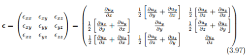
where if the displacement field is given a Lagrangian description we would use a Lagrangian gradient and if the displacement field is given a Eulerian description Eulerian gradient is used. Strictly speaking, we should only use the Eulerian gradient since this strain is to be related to the Cauchy stress.
Similarly the cylindrical polar components of the linearized strain are,
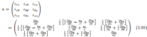
where we have made use of the expression (2.259) for finding the gradient of the displacement field in cylindrical coordinates.
Normal strain
The component of the strain that represents the changes in length along a given direction is called normal strain. From equation (3.89), the change in length along a given direction A is,
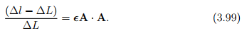
Thus, the change in length along coordinate basis directions - ex, ey, ez - is given by the components - exx, eyy, ezz - respectively. Therefore these components are called as the normal strian components
Principal strain
Of interest is the maximum change in length that occurs in the body subjected to a given force and the direction in which this maximum change in length occurs. Thus, we need to find the vector A such that ║A║ = 1 and it maximizes, ∈(A) defined as,
∈(A) = ∈A · A. (3.100)
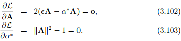
This constrained optimization is done by what is called as the Lagrangemultiplier method. Towards this, we introduce the function

where α* is the Lagrange multiplier and the condition ║A║2 − 1 = 0 characterizes the constraint condition. At locations where the extremal values of L occurs, the derivatives
 must vanish, i.e.,
To obtain these equations we have made use of the fact that linearized strain tensor is symmetric. Thus, we have to find three Âa and α*a ’s such that

(a = 1, 2, 3; no summation) which is nothing but the eigenvalue problem involving the tensor ∈ with the Lagrange multiplier being identified as the eigenvalue. Hence, the results of section 2.5 follows. In particular, for (3.104a) to have a non-trivial solution

where

the principal invariants of the strain ∈. As stated in section 2.5, equation (3.105 has three real roots, since the linearized strain tensor is symmetric.
These roots (α*a ) will henceforth be denoted by ∈1, ∈2 and ∈3 and are called principal strains. The principal strains include both the maximum and minimum normal strains among all material fibers passing through a given x.
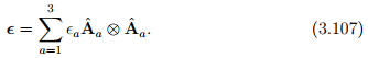
The corresponding three orthonormal eigenvectors Âa, which are then characterized through the relation (3.104) are called the principal directions of ∈. Further, these eigenvectors form a mutually orthogonal basis since the strain tensor ∈ is symmetric. This property of the strain tensor also allows us to represent ∈ in the spectral form
Shear strain
As we did to obtain equation (3.89) when the components of the displacement gradient are small, the right Cauchy-Green deformation tensor could be approximately computed as, C ≈ 1 + 2∈. For this approximation, the deformed angle between two line segments initially oriented along A1 and A2 directions given in (3.66) simplifies to,
cos(αf ) = A1 · A2 + 2∈A1 · A2, (3.108)
where we have approximated (1 + 2 ∈A · A) as 1, since the components of ∈ is much less than 1 (of the order of 10−3 ) and the components of A is less than or equal to 1. If α is the angle between the line elements in the reference configuration, then cos(α) = A1 · A2. Using the trigonometric relation, cos(A) − cos(B) = 2 sin((A + B)/2) sin((B − A)/2) and the assumption that the change in angle, αf − α, is small, equation (3.108) could be written as,
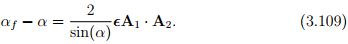
When A1 and A2 are identified with the orthonormal coordinate basis, then sin(α) = 1 and ∈A1 · A2 represents the off diagonal terms in the matrix representation of the components of the strain tensor. Hence, the off diagonal terms are the shear strains which represents half of the change in angle between orthogonal line elements oriented along the coordinate basis directions.
Therefore, we conclude that the diagonal elements in the matrix representation of the components of the strain tensor are related to the changes
in length of line elements oriented along the direction of the orthonormal coordinate basis and the off diagonal elements are related to the changes in angle of these line elements oriented along the direction of the orthonormal basis. We also infer that there is no change in angle between line elements along which the change in length is a extremum. This is a consequence of the observation that the off diagonal elements are zero in the equation (3.107) representing the strain using the principal directions as the coordinate basis.
Transformation of linearized strain tensor
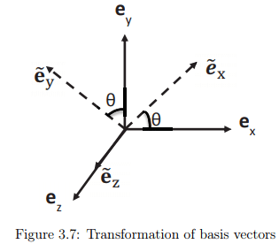
Now, we are interested in finding how the components of the linearized strain change due to transformation of the coordinate basis. By virtue of the linearized strain being a second order tensor, the transformation laws (2.161) derived in section 2.6.2 hold. Thus, if Qij (= ei · êj ) represents the directional cosine matrix of the transformation from coordinate basis {e1, e2, e3} to the basis {ê1, ê2, ê3}, then the strain components in the êi basis,  could be obtained from the strain components in the ei basis, ∈ij , through the equation,
= ∈abQaiQbj . (3.110)
Let us specialize to a state of strain wherein the strain tensor has a representation,
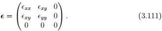
This state of strain is called as plane strain. A state of strain is said to be plane strain if at least one of its principal values is zero which means that det( ∈) = 0. Let us further assume that êj is related to ei through,

This represents a anticlockwise rotation of the ei basis about e3 basis to obtain the new basis vectors (see figure 3.7). Substituting equations (3.111) and (3.112) in (3.110) we obtain,
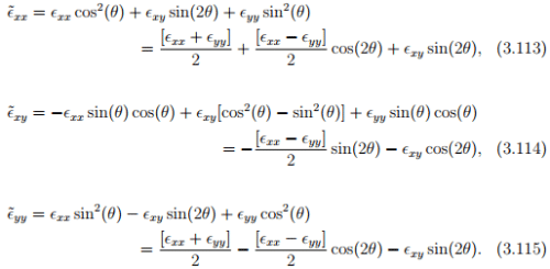
These set of equations is what is popularly called as Mohr’s equations. The fact that this is for a special state of strain and special transformation of the coordinate basis cannot be overemphasized.


