Linear Programming (Part - 3) - Electronics and Communication Engineering (ECE) PDF Download

Linear Programming - Part - 3, Operations Research
The Big M Method
If an LP has any ≥ or = constraints, a starting bfs may not be readily apparent. When a bfs is not readily apparent, the Big M method or the two-phase simplex method may be used to solve the problem.
The Big M method is a version of the Simplex Algorithm that first finds a bfs by adding "artificial" variables to the problem. The objective function of the original LP must, of course, be modified to ensure that the artificial variables are all equal to 0 at the conclusion of the simplex algorithm.
Steps
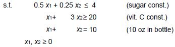
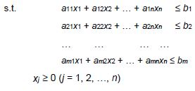
1. Modify the constraints so that the RHS of each constraint is nonnegative (This requires that each constraint with a negative RHS be multiplied by -1. Remember that if you multiply an inequality by any negative number, the direction of the inequality is reversed!). After modification, identify each constraint as a ≤, ≥ or = constraint.
2. Convert each inequality constraint to standard form (If constraint i is a ≤ constraint, we add a slack variable si; and if constraint i is a ≥ constraint, we subtract an excess variable ei).
3. Add an artificial variable ai to the constraints identified as ≥ or = constraints at the end of Step 1. Also add the sign restriction ai ≥ 0.
4. Let M denote a very large positive number. If the LP is a min problem, add (for each artificial variable) Mai to the objective function. If the LP is a max problem, add (for each artificial variable) -Mai to the objective function.
5. Since each artificial variable will be in the starting basis, all artificial variables must be eliminated from row 0 before beginning the simplex. Now solve the transformed problem by the simplex (In choosing the entering variable, remember that M is a very large positive number!).
If all artificial variables are equal to zero in the optimal solution, we have found the optimal solution to the original problem.
If any artificial variables are positive in the optimal solution, the original problem is infeasible!!!
Example 1. Oranj Juice
(Winston 4.10, p. 164)
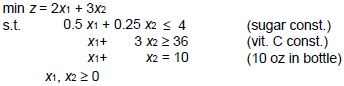
Bevco manufactures an orange flavored soft drink called Oranj by combining orange soda and orange juice. Each ounce of orange soda contains 0.5 oz of sugar and 1 mg of vitamin C. Each ounce of orange juice contains 0.25 oz of sugar and 3 mg of vitamin C. It costs Bevco 2¢ to produce an ounce of orange soda and 3¢ to produce an ounce of orange juice. Marketing department has decided that each 10 oz bottle of Oranj must contain at least 20 mg of vitamin C and at most 4 oz of sugar. Use LP to determine how Bevco can meet marketing dept.’s requirements at minimum cost.
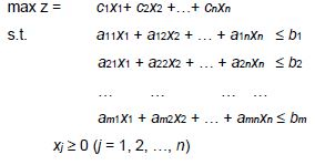
LP Model:
Let x1 and x2 be the quantity of ounces of orange soda and orange juice (respectively) in a bottle of Oranj.
min z = 2x1 + 3x2
Solving Oranj Example with Big M Method
1. Modify the constraints so that the RHS of each constraint is nonnegative The RHS of each constraint is nonnegative
2. Convert each inequality constraint to standard form
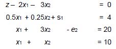
all variables nonnegative
3. Add ai to the constraints identified as > or = const.s
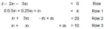
all variables nonnegative
4. Add Mai to the objective function (min problem)
min z = 2x1 + 3x2 + Ma2 + Ma3
Row 0 will change to
z – 2x1 – 3x2 – Ma2 – Ma3 = 0
5. Since each artificial variable are in our starting bfs, they must be eliminated from row 0
New Row 0 = Row 0 + M * Row 2 + M * Row 3 ⇒
z + (2M–2) x1 + (4M–3) x2 – M e2 = 30M New Row 0
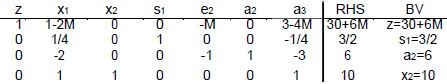
Initial tableau:
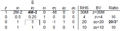
In a min problem, entering variable is the variable that has the “most positive” coefficient in row 0!
First tableau:
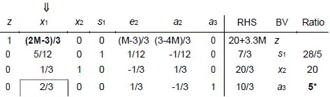
Optimal tableau:
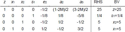
Report:
In a bottle of Oranj, there should be 5 oz orange soda and 5 oz orange juice.
In this case the cost would be 25¢.
Example 2. Modified Oranj Juice
Consider Bevco’s problem. It is modified so that 36 mg of vitamin C are required.
Related LP model is given as follows:
Let x1 and x2 be the quantity of ounces of orange soda and orange juice (respectively) in a bottle of Oranj.
Solving with Big M method:
Initial tableau: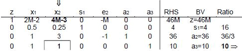
Optimal tableau:
An artificial variable (a2) is BV so the original LP has no feasible solution
Report:
It is impossible to produce Oranj under these conditions.
DUALITY
Primal – Dual
Associated with any LP is another LP called the dual. Knowledge of the dual provides interesting economic and sensitivity analysis insights. When taking the dual of any LP, the given LP is referred to as the primal. If the primal is a max problem, the dual will be a min problem and vice versa.
Finding the Dual of an LP
The dual of a normal max problem is a normal min problem.
Normal max problem is a problem in which all the variables are required to be nonnegative and all the constraints are ≤ constraints.
Normal min problem is a problem in which all the variables are required to be nonnegative and all the constraints are ≥ constraints.
Similarly, the dual of a normal min problem is a normal max problem.
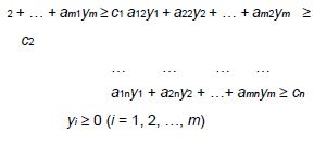
Finding the Dual of a Normal Max
Problem PRIMAL
DUAL
Finding the Dual of a Normal Min Problem
PRIMAL
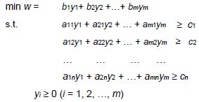
DUAL
max z = c1x1+ c2x2 +…+ cnxn
Finding the Dual of a Nonnormal Max Problem
- If the ith primal constraint is a ≥ constraint, the corresponding dual variable yi must satisfy yi ≤ 0
- If the ith primal constraint is an equality constraint, the dual variable yi is now unrestricted in sign (urs).
- If the ith primal variable is urs, the ith dual constraint will be an equality constraint
- Finding the Dual of a Nonnormal Min Problem
- If the ith primal constraint is a ≤ constraint, the corresponding dual variable xi must satisfy xi ≤ 0
- If the ith primal constraint is an equality constraint, the dual variable xi is now urs.
- If the ith primal variable is urs, the ith dual constraint will be an equality constraint
The Dual Theorem
The primal and dual have equal optimal objective function values (if the problems have optimal solutions).
Weak duality implies that if for any feasible solution to the primal and an feasible solution to the dual, the w-value for the feasible dual solution will be at least as large as the z-value for the feasible primal solution z ≤ w.
Consequences
- Any feasible solution to the dual can be used to develop a bound on the optimal value of the primal objective function.
- If the primal is unbounded, then the dual problem is infeasible.
- If the dual is unbounded, then the primal is infeasible.
- How to read the optimal dual solution from Row 0 of the optimal tableau if the primal is a max problem:
‘optimal value of dual variable yi’
= ‘coefficient of si in optimal row 0’ (if const. i is a ≤ const.)
= –‘coefficient of ei in optimal row 0’ (if const. i is a ≥ const.)
= ‘coefficient of ai in optimal row 0’ – M (if const. i is a = const.)
- How to read the optimal dual solution from Row 0 of the optimal tableau if the primal is a min problem:
‘optimal value of dual variable xi’
= ‘coefficient of si in optimal row 0’
(if const. i is a ≤ const.)
= –‘ coefficient of ei in optimal row 0’
(if const. i is a ≥ const.)
= ‘coefficient of ai in optimal row 0’ + M
(if const. i is a = const.)
Economic Interpretation
When the primal is a normal max problem, the dual variables are related to the value of resources available to the decision maker. For this reason, dual variables are often referred to as resource shadow prices.
Example
PRIMAL
Let x1, x2, x3 be the number of desks, tables and chairs produced. Let the weekly profit be $z. Then, we must
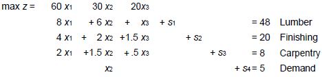
max z = 60x1 + 30x2 + 20x3
8x1 + 6x2 + x3 ≤ 48 (Lumber constraint)
4x1 + 2x2 + 1.5x3 ≤ 20 (Finishing hour constraint)
2x1 + 1.5x2 + 0.5x3 ≤ 8 (Carpentry hour constraint)
x1, x2, x3 ≥ 0
DUAL
Suppose an entrepreneur wants to purchase all of Dakota’s resources.
In the dual problem y1, y2, y3 are the resource prices (price paid for one board ft of lumber, one finishing hour, and one carpentry hour). $w is the cost of purchasing the resources.
Resource prices must be set high enough to induce Dakota to sell. i.e. total purchasing cost equals total profit.
min w = 48y1 + 20y2 +8y3
s.t.
8y1 +4y2+2y3≥60 (Desk constraint)
6y1 +2y2+ 1.5y3≥30 (Table constraint)
y1 + 1.5y2+ 0.5y3≥20 (Chair constraint)
y1, y2, y3 ≥ 0
SENSITIVITY ANALYSIS
Reduced Cost
For any nonbasic variable, the reduced cost for the variable is the amount by which the nonbasic variable's objective function coefficient must be improved before that variable will become a basic variable in some optimal solution to the LP.
If the objective function coefficient of a nonbasic variable xk is improved by its reduced cost, then the LP will have alternative optimal solutions at least one in which xk is a basic variable, and at least one in which xk is not a basic variable.
If the objective function coefficient of a nonbasic variable xk is improved by more than its reduced cost, then any optimal solution to the LP will have xk as a basic variable and xk > 0.
Reduced cost of a basic variable is zero (see definition)!
Shadow Price
We define the shadow price for the ith constraint of an LP to be the amount by which the optimal z value is "improved" (increased in a max problem and decreased in a min problem) if the RHS of the ith constraint is increased by 1.
This definition applies only if the change in the RHS of the constraint leaves the current basis optimal!
A ≥ constraint will always have a nonpositive shadow price; a ≤ constraint will always have a nonnegative shadow price.
Conceptualization
max z = 5 x1 + x2 + 10x3
x1 + x3 ≤ 100
x2 ≤ 1
All variables ≥ 0
This is a very easy LP model and can be solved manually without utilizing Simplex.
x2 = 1 (This variable does not exist in the first constraint. In this case, as the problem is a maximization problem, the optimum value of the variable equals the RHS value of the second constraint).
x1 = 0, x3 = 100 (These two variables do exist only in the first constraint and as the objective function coefficient of x3 is greater than that of x1, the optimum value of x3 equals the RHS value of the first constraint). Hence, the optimal solution is as follows:
z = 1001, [x1, x2, x3] = [0, 1, 100]
Similarly, sensitivity analysis can be executed manually.
Reduced Cost
As x2 and x3 are in the basis, their reduced costs are 0.
In order to have x1 enter in the basis, we should make its objective function coefficient as great as that of x3. In other words, improve the coefficient as 5 (10-5). New objective function would be (max z = 10x1 + x2 + 10x3) and there would be at least two optimal solutions for [x1, x2, x3]: [0, 1, 100] and [100, 1, 0]. Therefore reduced cost of x1 equals 5.
If we improve the objective function coefficient of x1 more than its reduced cost, there would be a unique optimal solution: [100, 1, 0].
Shadow Price
If the RHS of the first constraint is increased by 1, new optimal solution of x3 would be 101 instead of 100. In this case, new z value would be 1011.
If we use the definition: 1011 - 1001 = 10 is the shadow price of the first constraint. Similarly the shadow price of the second constraint can be calculated as 1 (please find it).
Utilizing Lindo Output for Sensitivity
NOTICE: The objective function which is regarded as Row 0 in Simplex is accepted as Row 1 in Lindo.
Therefore the first constraint of the model is always second row in Lindo!!!
MAX 5 X1 + X2 + 10 X3
SUBJECT TO
2) X1 + X3 <= 100
3) X2 <= 1
END
LP OPTIMUM FOUND AT STEP
OBJECTIVE FUNCTION VALUE
1) 1001.000
RANGES IN WHICH THE BASIS IS UNCHANGED:
OBJ COEFFICIENT RANGES
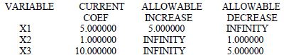
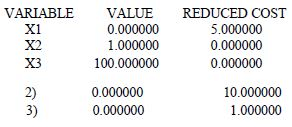
Lindo output reveals the reduced costs of x1, x2, and x3 as 5, 0, and 0 respectively.
In the maximization problems, the reduced cost of a non-basic variable can also be read from the allowable increase value of that variable at obj. coefficient ranges. Here, the corresponding value of x1 is 5.
In the minimization problems, the reduced cost of a non-basic variable can also be read from the allowable decrease value of that variable at obj. coefficient ranges. The same Lindo output reveals the shadow prices of the constraints in the "dual price" section:
Here, the shadow price of the first constraint (Row 2) equals 10.
The shadow price of the second constraint (Row 3) equals 1.
Some important equations
If the change in the RHS of the constraint leaves the current basis optimal (within the allowable RHS range), the following equations can be used to calculate new
objective function value:
for maximization problems
- new obj. fn. value = old obj. fn. value + (new RHS – old RHS) × shadow price for minimization problems
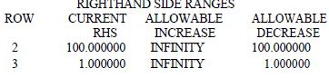
- new obj. fn. value = old obj. fn. value – (new RHS – old RHS) × shadow price For Lindo example, as the allowable increases in RHS ranges are infinity for each constraint, we can increase RHS of them as much as we want. But according to allowable decreases, RHS of the first constraint can be decreased by 100 and that of second constraint by 1
Lets assume that new RHS value of the first constraint is 60.
As the change is within allowable range, we can use the first equation (max. problem):
znew = 1001 + ( 60 - 100 ) 10 = 601.
Utilizing Simplex for Sensitivity
In Dakota furniture example; x1, x2, and x3 were representing the number of desks, tables, and chairs produced.
The LP formulated for profit maximization:
The optimal solution was:
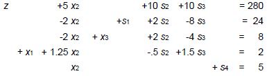
Analysis 1
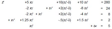
Suppose available finishing time changes from 20 → 20+δ, then we have the system:
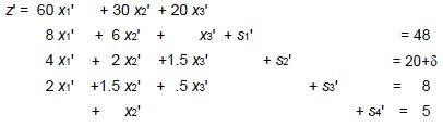
or equivalently
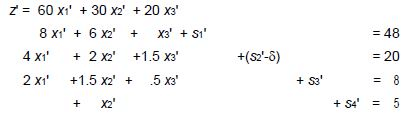
That is z, x1, x2, x3,x4,s1,s2 -δ,s3,s4 satisfy the original problem, and hence (1)
Substituting in:
and thus
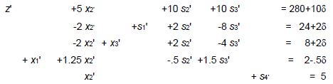
For -4 ≤ δ ≤4, the new system maximizes z’. In this range RHS values are non-negative.
As δ increases, revenue increases by 10 δ. Therefore, the shadow price of finishing labor is $10 per hr. (This is valid for up to 4 extra hours or 4 fewer hours).
Analysis 2
What happens if revenue from desks changes to $60+ γ? For small γ revenue increases by 2 γ (as we are making 2 desks currently). But how large an increase is possible?
The new revenue is:
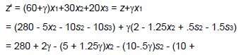
1.5γ)s3 So the top line in the final system would be:
z' + (5 + 1.25γ)x2 + (10 - .5γ)s2 + (10 + 1.5γ)s3 = 280 +
2γ Provided all terms in this row are ≥0 we are still optimal. For -4 ≤ γ ≤ 20, the current production schedule is still optimal.
Analysis 3
If revenue from a non-basic variable changes, the revenue is
z’ = 60x1 + (30 + γ)x2 + 20x3 = z + γx2
= 280 - 5x2 - 10s2 - 10s3 + γx2
= 280 - (5 - γ)x2 - 10s2 - 10s3
The current solution is optimal for γ ≤ 5. But when > 5 or the revenue per table is increased past $35, it becomes better to produce tables. We say the reduced cost of tables is $5.00.
Duality and Sensitivity Analysis
Will be treated at the class.
The 100% Rule
Will be treated at the class.
FAQs on Linear Programming (Part - 3) - Electronics and Communication Engineering (ECE)
| 1. What is linear programming and how is it used in various industries? |  |
| 2. What are the key components of a linear programming problem? | |
| 3. How do you formulate a linear programming problem? | |
| 4. Can linear programming be used for solving real-world problems? | |
| 5. What are the limitations of linear programming? | |


Top Courses for Electronics and Communication Engineering (ECE)
Linear Programming (Part - 3) - Electronics and Communication Engineering (ECE)
,video lectures
,Exam
,Free
,Previous Year Questions with Solutions
,shortcuts and tricks
,Sample Paper
,Summary
,study material
,practice quizzes
,past year papers
,ppt
,Extra Questions
,Viva Questions
,Objective type Questions
,Linear Programming (Part - 3) - Electronics and Communication Engineering (ECE)
,Important questions
,Linear Programming (Part - 3) - Electronics and Communication Engineering (ECE)
,Semester Notes
,MCQs
,mock tests for examination
;


Linear Programming (Part - 3) Free PDF Download
Importance of Linear Programming (Part - 3)
Linear Programming (Part - 3) Notes
Linear Programming (Part - 3) Electronics and Communication Engineering (ECE) Questions
Study Linear Programming (Part - 3) on the App
|
© EduRev
|
Education Revolution
|


|


within 7 days!