Transportation Problem (Part - 2) - Electronics and Communication Engineering (ECE) PDF Download

Transportation Problem - Part - 2, Operations Research
THE TRANSPORTATION SIMPLEX METHOD
Steps of the Method
1. If the problem is unbalanced, balance it
2. Use one of the methods to find a bfs for the problem
3. Use the fact that u1 = 0 and ui + vj = cij for all basic variables to find the u’s and v’s for the current bfs.
4. If ui + vj – cij ≤ 0 for all nonbasic variables, then the current bfs is optimal. If this is not the case, we enter the variable with the most positive ui + vj – cij into the basis using the pivoting procedure. This yields a new bfs. Return to Step 3.
For a maximization problem, proceed as stated, but replace Step 4 by the following step:
If ui + vj – cij ≥ 0 for all nonbasic variables, then the current bfs is optimal. Otherwise, enter the variable with the most negative ui + vj – cij into the basis using the pivoting procedure. This yields a new bfs. Return to Step 3.
Pivoting procedure
1. Find the loop (there is only one possible loop!) involving the entering variable (determined at step 4 of the transport’n simplex method) and some or all of the basic variables.
2. Counting only cells in the loop, label those that are an even number (0, 2, 4, and so on) of cells away from the entering variable as even cells. Also label those that are an odd number of cells away from the entering variable as odd cells.
3. Find the odd cell whose variable assumes the smallest value. Call this value φ. The variable corresponding to this odd cell will leave the basis. To perform the pivot, decrease the value of each odd cell by φ and increase the value of each even cell by φ. The values of variables not in the loop remain unchanged. The pivot is now complete. If φ = 0, the entering variable will equal 0, and odd variable that has a current value of 0 will leave the basis.
Example 1. Powerco
The problem is balanced (total supply equals total demand).
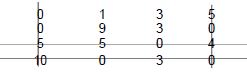
When the NWC method is applied to the Powerco example, the bfs in the following table is obtained (check: there exist m+n–1=6 basic variables).
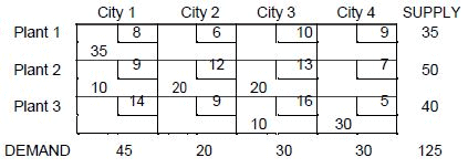
u1= 0
u1+ v1 = 8 yields v1 = 8
u2+ v1 = 9 yields u2 = 1
u2+ v2 = 12 yields v2 = 11
u2+ v3 = 13 yields v3 = 12
u3+ v3 = 16 yields u3 = 4
u3+ v4 = 5 yields v4 = 1
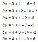
Since ĉ32 is the most positive one, we would next enter x32 into the basis: Each unit of x32 that is entered into the basis will decrease Powerco’s cost by $6.
The loop involving x32 is (3,2)-(3,3)-(2,3)-(2,2). φ = 10 (see table)
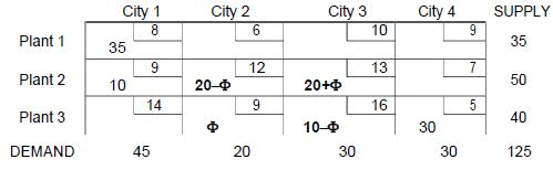
x33 would leave the basis. New bfs is shown at the following table:
Since ĉ12 is the most positive one, we would next enter x12 into the basis.
The loop involving x12 is (1,2)-(2,2)-(2,1)-(1,1). φ = 10 (see table)
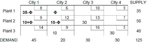
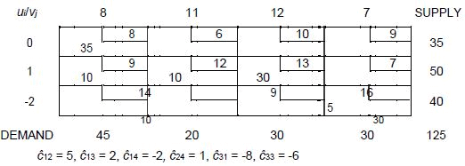
x22 would leave the basis. New bfs is shown at the following table
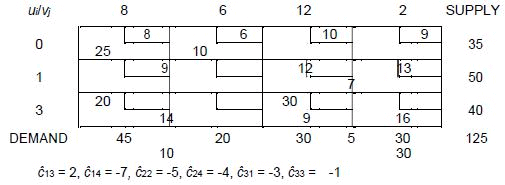
Since ĉ13 is the most positive one, we would next enter x13 into the basis.
The loop involving x13 is (1,3)-(2,3)-(2,1)-(1,1). φ = 25 (see table)
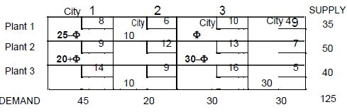
x11 would leave the basis. New bfs is shown at the following table:
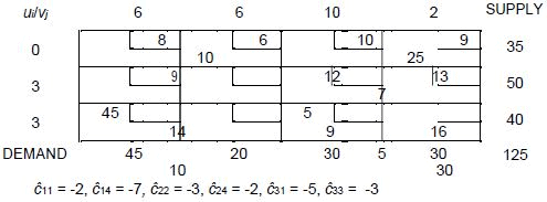
Since all ĉij’s are negative, an optimal solution has been obtained.
Report
45 million kwh of electricity would be sent from plant 2 to city 1.
10 million kwh of electricity would be sent from plant 1 to city 2. Similarly, 10 million kwh of electricity would be sent from plant 3 to city 2.
25 million kwh of electricity would be sent from plant 1 to city 3. 5 million kwh of electricity would be sent from plant 2 to city 3.
30 million kwh of electricity would be sent from plant 3 to city 4 and
Total shipping cost is:
z = .9 (45) + 6 (10) + 9 (10) + 10 (25) + 13 (5) + 5 (30) = $ 1020
TRANSSHIPMENT PROBLEMS
Sometimes a point in the shipment process can both receive goods from other points and send goods to other points. This point is called as transshipment point through which goods can be transshipped on their journey from a supply point to demand point.
Shipping problem with this characteristic is a transshipment problem.
The optimal solution to a transshipment problem can be found by converting this transshipment problem to a transportation problem and then solving this transportation problem.
Remark
As stated in “Formulating Transportation Problems”, we define a supply point to be a point that can send goods to another point but cannot receive goods from any other point.
Similarly, a demand point is a point that can receive goods from other points but cannot send goods to any other point.
Steps
1. If the problem is unbalanced, balance it
Let s = total available supply (or demand) for balanced problem
2. Construct a transportation tableau as follows
A row in the tableau will be needed for each supply point and transshipment point A column will be needed for each demand point and transshipment point
Each supply point will have a supply equal to its original supply Each demand point will have a demand equal to its original demand
Each transshipment point will have a supply equal to “that point’s original supply + s”
Each transshipment point will have a demand equal to “that point’s original demand + s”
3. Solve the transportation problem
Example 1. Bosphorus
(Based on Winston 7.6.)
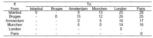
Bosphorus manufactures LCD TVs at two factories, one in Istanbul and one in Bruges. The Istanbul factory can produce up to 150 TVs per day, and the Bruges factory can produce up to 200 TVs per day. TVs are shipped by air to customers in London and Paris. The customers in each city require 130 TVs per day. Because of the deregulation of air fares, Bosphorus believes that it may be cheaper to first fly some TVs to Amsterdam or Munchen and then fly them to their final destinations.
The costs of flying a TV are shown at the table below. Bosphorus wants to minimize the total cost of shipping the required TVs to its customers.
Answer:
In this problem Amsterdam and Munchen are transshipment points.
Step 1. Balancing the problem
Total supply = 150 + 200 = 350
Total demand = 130 + 130 = 260
Dummy’s demand = 350 – 260 = 90
s = 350 (total available supply or demand for balanced problem)
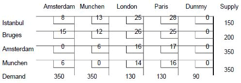
Step 2. Constructing a transportation tableau
Transshipment point’s demand = Its original demand + s = 0 + 350 = 350 Transshipment point’s supply = Its original supply + s = 0 + 350 = 350
Step 3. Solving the transportation problem
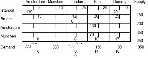
Report:
Bosphorus should produce 130 TVs at Istanbul, ship them to Amsterdam, and transship them from Amsterdam to London.
The 130 TVs produced at Bruges should be shipped directly to Paris.
The total shipment is 6370 Euros.
ASSIGNMENT PROBLEMS
There is a special case of transportation problems where each supply point should be assigned to a demand point and each demand should be met. This certain class of problems is called as “assignment problems”. For example determining which employee or machine should be assigned to which job is an assignment problem.
LP Representation
An assignment problem is characterized by knowledge of the cost of assigning each supply point to each demand point: cij
On the other hand, a 0-1 integer variable xij is defined as follows
xij = 1 if supply point i is assigned to meet the demands of demand point j xij = 0 if supply point i is not assigned to meet the demands of point j
In this case, the general LP representation of an assignment problem is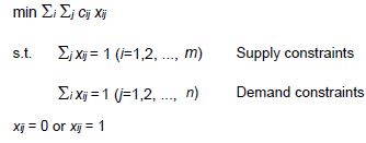
Hungarian Method
Since all the supplies and demands for any assignment problem are integers, all variables in optimal solution of the problem must be integers. Since the RHS of each constraint is equal to 1, each xij must be a nonnegative integer that is no larger than 1, so each xij must equal 0 or 1.
Ignoring the xij = 0 or xij = 1 restrictions at the LP representation of the assignment problem, we see that we confront with a balanced transportation problem in which each supply point has a supply of 1 and each demand point has a demand of 1.
However, the high degree of degeneracy in an assignment problem may cause the Transportation Simplex to be an inefficient way of solving assignment problems.
For this reason and the fact that the algorithm is even simpler than the Transportation Simplex, the Hungarian method is usually used to solve assignment problems.
Remarks
1. To solve an assignment problem in which the goal is to maximize the objective function, multiply the profits matrix through by –1 and solve the problem as a minimization problem.
2. If the number of rows and columns in the cost matrix are unequal, the assignment problem is unbalanced. Any assignment problem should be balanced by the addition of one or more dummy points before it is solved by the Hungarian method.
Steps
1. Find the minimum cost each row of the m*m cost matrix.
2. Construct a new matrix by subtracting from each cost the minimum cost in its row
3. For this new matrix, find the minimum cost in each column
4. Construct a new matrix (reduced cost matrix) by subtracting from each cost the minimum cost in its column
5. Draw the minimum number of lines (horizontal and/or vertical) that are needed to cover all the zeros in the reduced cost matrix. If m lines are required, an optimal solution is available among the covered zeros in the matrix. If fewer than m lines are needed, proceed to next step
6. Find the smallest cost (k) in the reduced cost matrix that is uncovered by the lines drawn in Step 5
7. Subtract k from each uncovered element of the reduced cost matrix and add k to each element that is covered by two lines. Return to Step 5
Example 1. Flight Crew
(Based on Winston 7.5.)
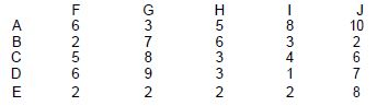
Four captain pilots (CP1, CP2, CP3, CP4) has evaluated four flight officers (FO1, FO2, FO3, FO4) according to perfection, adaptation, morale motivation in a 1-20 scale (1: very good, 20: very bad). Evaluation grades are given in the table. Flight Company wants to assign each flight officer to a captain pilot according to these evaluations. Determine possible flight crews.
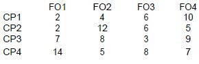
Answer:
Step 1. For each row in the table we find the minimum cost: 2, 2, 3, and 5 respectively
Step 2 & 3. We subtract the row minimum from each cost in the row. For this new matrix, we find the minimum cost in each column
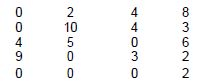
Step 4. We now subtract the column minimum from each cost in the column obtaining reduced cost matrix.
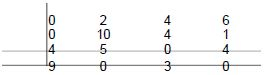
Step 5. As shown, lines through row 3, row 4, and column 1 cover all the zeros in the reduced cost matrix. The minimum number of lines for this operation is 3. Since fewer than four lines are required to cover all the zeros, solution is not optimal: we proceed to next step.
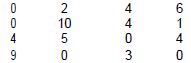
Step 6 & 7. The smallest uncovered cost equals 1. We now subtract 1 from each uncovered cost, add 1 to each twice-covered cost, and obtain
Four lines are now required to cover all the zeros: An optimal s9olution is available. Observe that the only covered 0 in column 3 is x33, and in column 2 is x42. As row 5 can not be used again, for column 4 the remaining zero is x24. Finally we choose x11.
Report:
CP1 should fly with FO1; CP2 should fly with FO4; CP3 should fly with FO3; and CP4 should fly with FO4.
Example 2. Maximization problem
Report:
Optimal profit = 36
Assigments: A-I, B-H, C-G, D-F, E-J
Alternative optimal sol’n: A-I, B-H, C-F, D-G, E-J
FAQs on Transportation Problem (Part - 2) - Electronics and Communication Engineering (ECE)
| 1. What is a transportation problem? |  |
| 2. How can a transportation problem be formulated? | |
| 3. What are the key components of a transportation problem? | |
| 4. How is the optimal solution found in a transportation problem? | |
| 5. What are some practical applications of transportation problems? | |


Top Courses for Electronics and Communication Engineering (ECE)
Transportation Problem (Part - 2) - Electronics and Communication Engineering (ECE)
,Extra Questions
,past year papers
,Important questions
,Transportation Problem (Part - 2) - Electronics and Communication Engineering (ECE)
,study material
,MCQs
,shortcuts and tricks
,video lectures
,ppt
,Summary
,practice quizzes
,Previous Year Questions with Solutions
,Semester Notes
,Viva Questions
,Sample Paper
,Transportation Problem (Part - 2) - Electronics and Communication Engineering (ECE)
,Free
,Exam
,Objective type Questions
,mock tests for examination
;


Transportation Problem (Part - 2) Free PDF Download
Importance of Transportation Problem (Part - 2)
Transportation Problem (Part - 2) Notes
Transportation Problem (Part - 2) Electronics and Communication Engineering (ECE) Questions
Study Transportation Problem (Part - 2) on the App
|
© EduRev
|
Education Revolution
|


|


