Synchronous Motor - 2 | Electrical Engineering SSC JE (Technical) - Electrical Engineering (EE) PDF Download
Synchronous-motor power equation
Except for very small machines, the armature resistance of a synchronous motor is relatively insignificant compared to its synchronous reactance, so that Eqn. 61 to be approximated to
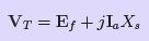 (62)
(62)
The equivalent-circuit and phasor diagram corresponding to this relation are shown in Fig. 54 and Fig. 55. These are normally used for analyzing the behavior of a synchronous motor, due to changes in load and/or changes in field excitation.
From this phasor diagram, we have,
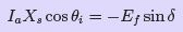 (63)
(63)
Multiplying through by VT and rearranging terms we have,
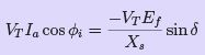 (64)
(64)
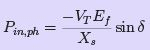
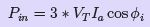
Since the left side of Eqn. 64 is an expression for active power input and as the winding resistance is assumed to be negligible this power input will also represent the electromagnetic power developed, per phase, by the synchronous motor.
Thus,
 (65)
(65)
or
 (66)
(66)
Thus, for a three-phase synchronous motor,
 (67)
(67)
or
 (68)
(68)
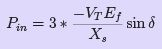
Eqn. 66, called the synchronous-machine power equation, expresses the electro magnetic power developed per phase by a cylindrical-rotor motor, in terms of its excitation voltage and power angle. Assuming a constant source voltage and constant supply frequency, Eqn. 65 and Eqn. 66 may be expressed as proportionalities that are very useful for analyzing the behavior of a synchronous-motor:
 (69)
(69)
 (70)
(70)
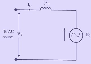
Figure 54: Equivalent-circuit of a synchronous-motor, assuming armature resistance is negligible
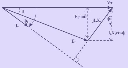
Figure 55: Phasor diagram model for a synchronous-motor, assuming armature resistance is negligible
Effect of changes in load on armature current, power angle, and power factor of synchronous motor
The effects of changes in mechanical or shaft load on armature current, power angle, and power factor can be seen from the phasor diagram shown in Fig. 56; As already stated, the applied stator voltage, frequency, and field excitation are assumed, constant. The initial load conditions, are represented by the thick lines. The effect of increasing the shaft load to twice its initial value are represented by the light lines indicating the new steady state conditions. These are drawn in accordance with Eqn. 69 and Eqn. 70, when the shaft load is doubled both Ia cos φi and Ef sin δ are doubled. While redrawing the phasor diagrams to show new steady-state conditions, the line of action of the new j IaXs phasor must be perpendicular to the new Ia phasor. Furthermore, as shown in Fig. 56, if the excitation is not changed, increasing the shaft load causes the locus of the Ef phasor to follow a circular arc, thereby increasing its phase angle with increasing shaft load. Note also that an increase in shaft load is also accompanied by a decrease in φi; resulting in an increase in power factor.
As additional load is placed on the machine, the rotor continues to increase its angle
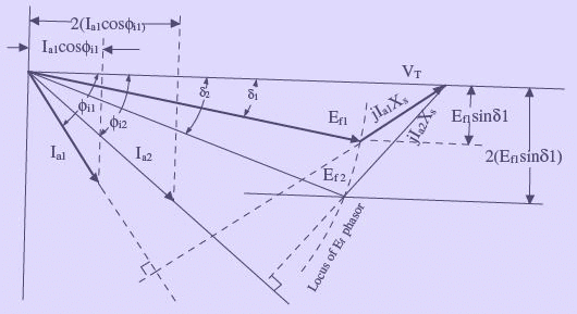
Figure 56: Phasor diagram showing effect of changes in shaft load on armature current, power angle and power factor of a synchronous motor
of lag relative to the rotating magnetic field, thereby increasing both the angle of lag of the counter EMF phasor and the magnitude of the stator current. It is interesting to note that during all this load variation, however, except for the duration of transient conditions whereby the rotor assumes a new position in relation to the rotating magnetic field, the average speed of the machine does not change. As the load is being increased, a final point is reached at which a further increase in δ fails to cause a corresponding increase in motor torque, and the rotor pulls out of synchronism. In fact as stated earlier, the rotor poles at this point, will fall behind the stator poles such that they now come under the influence of like poles and the force of attraction no longer exists. Thus, the point of maximum torque occurs at a power angle of approximately 90◦ for a cylindrical-rotor machine, as is indicated by Eqn. 68. This maximum value of torque that causes a synchronous motor to pull out of synchronism is called the pull-out torque. In actual practice, the motor will never be operated at power angles close to 90◦ as armature current will be many times its rated value at this load.
Effect of changes in field excitation on synchronous motor performance
Intuitively we can expect that increasing the strength of the magnets will increase the magnetic attraction, and thereby cause the rotor magnets to have a closer alignment with the corresponding opposite poles of the rotating magnetic poles of the stator. This will obviously result in a smaller power angle. This fact can also be seen in Eqn. 68. When the shaft load is assumed to be constant, the steady-state value of Ef sin δ must also be constant. An increase in Ef will cause a transient increase in Ef sin δ, and the rotor will accelerate. As the rotor changes its angular position, δ decreases until Ef sin δ has the same steady-state value as before, at which time the rotor is again operating at synchronous speed, as it should run only at the synchronous speed. This change in angular position of the rotor magnets relative to the poles of rotating magnetic field of the stator occurs in a fraction of a second.
The effect of changes in field excitation on armature current, power angle, and power factor of a synchronous motor operating with a constant shaft load, from a constant voltage, constant frequency supply, is illustrated in Fig. 57. From Eqn. 69, we have for a constant shaft load,
 (71)
(71)
This is shown in Fig. 57, where the locus of the tip of the Ef phasor is a straight line parallel to the VT phasor. Similarly, from Eqn. 69, for a constant shaft load,
 (72)
(72)
This is also shown in Fig. 57, where the locus of the tip of the Ia phasor is a line
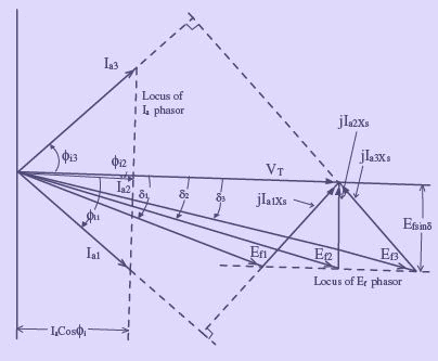
Figure 57: Phasor diagram showing effect of changes in field excitation on armature current, power angle and power factor of a synchronous motor perpendicular to the VT phasor.
Note that increasing the excitation from Ef 1 to Ef 3 in Fig. 57 caused the phase angle of the current phasor with respect to the terminal voltage VT (and hence the power factor) to go from lagging to leading. The value of field excitation that results in unity power factor is called normal excitation. Excitation greater than normal is called over excitation, and excitation less than normal is called under excitation. Furthermore, as indicated in Fig. 57, when operating in the overexcited mode, |Ef | > |VT |. In fact a synchronous motor operating under over excitation condition is sometimes called a synchronous condenser.
V curves
Curves of armature current vs. field current (or excitation voltage to a different scale) are called V curves, and are shown in Fig. 58 for typical values of synchronous motor loads. The curves are related to the phasor diagram in Fig. 57, and illustrate the effect of the variation of field excitation on armature current and power factor for typical shaft loads. It can be easily noted from these curves that an increase in shaft loads require an increase in field excitation in order to maintain the power factor at unity.
The locus of the left most point of the V curves in Fig. 58 represents the stability limit (δ = −90◦). Any reduction in excitation below the stability limit for a particular load will cause the rotor to pullout of synchronism.
The V curves shown in Fig. 58 can be determined experimentally in the laboratory by varying If at a constant shaft load and noting Ia as If is varied. Alternatively the V curves shown in Fig. 58 can be determined graphically by plotting |Ia|vs.|Ef | from a family of phasor diagrams as shown in Fig. 57, or from the following mathematical expression for the V curves
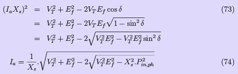
Eqn. 74 is based on the phasor diagram and the assumption that Ra is negligible. It is to be noted that instability will occur, if the developed torque is less than the shaft load plus friction and windage losses, and the expression under the square root sign will be negative.
The family of V curves shown in Fig. 58 represent computer plots of Eqn. 74, by taking the data pertaining to a three-phase 10 hp synchronous motor i.e Vph = 230V and Xs = 1.2Ω/phase.
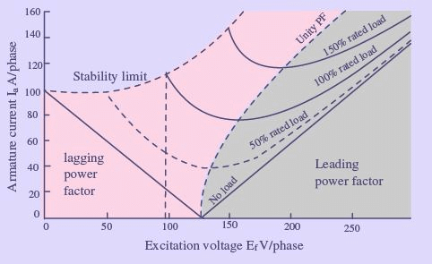
Figure 58: Family of representative V curves for a synchronous motor
Synchronous-motor losses and efficiency
The flow of power through a synchronous motor, from stator to rotor and then to shaft output, is shown in Fig. 59. As indicated in the power-flow diagram, the total power loss for the motor is given by
 (75)
(75)
where: Pscl= stator-copper loss
Pf cl = fie1d-copper.loss
Pcore = core loss
Pf,w = friction and windage loss
Pstray = stray load loss
Except for the transient conditions that occur when the field current is increased or decreased (magnetic energy stored or released), the total energy supplied to the field coils is constant and all of it is consumed as I 2R losses in the field winding. Just as in the case of the synchronous generator, the overall efficiency of a synchronous motor is given by
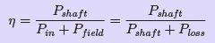 (76)
(76)
Generally, the nameplates of synchronous motors and manufacturers’ specification sheets customarily provide the overall efficiency for rated load and few load conditions only.
Hence, only the total losses at these loads can be determined. The separation of losses into the components listed in Eqn. 75 needs a very involved test procedure in the laboratory. However, a closer approximation of the mechanical power developed can be calculated by subtracting the copper losses of the armature and field winding if these losses can be calculated. The shaft power can then be calculated subtracting the mechanical losses from the mechanical power developed.
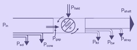
Figure 59: Power flow diagram for a synchronous motor
|
23 videos|89 docs|42 tests
|
FAQs on Synchronous Motor - 2 - Electrical Engineering SSC JE (Technical) - Electrical Engineering (EE)
| 1. What is a synchronous motor and how does it work? |  |
| 2. What are the advantages of using a synchronous motor? | |
| 3. How is the speed of a synchronous motor determined? | |
| 4. What are the main applications of synchronous motors? | |
| 5. How does a synchronous motor differ from an induction motor? | |

|
4.98/5 Rating |

|
Dec 22, 2024 Last updated |
|
23 videos|89 docs|42 tests
|

|
Explore Courses for Electrical Engineering (EE) exam
|
|
Viva Questions
,shortcuts and tricks
,Previous Year Questions with Solutions
,mock tests for examination
,Free
,Important questions
,Extra Questions
,Objective type Questions
,Semester Notes
,Synchronous Motor - 2 | Electrical Engineering SSC JE (Technical) - Electrical Engineering (EE)
,practice quizzes
,Summary
,video lectures
,Synchronous Motor - 2 | Electrical Engineering SSC JE (Technical) - Electrical Engineering (EE)
,ppt
,Synchronous Motor - 2 | Electrical Engineering SSC JE (Technical) - Electrical Engineering (EE)
,past year papers
,Exam
,study material
,Sample Paper
,MCQs
;


Synchronous Motor - 2 Free PDF Download
Importance of Synchronous Motor - 2
Synchronous Motor - 2 Notes
Synchronous Motor - 2 Electrical Engineering (EE) Questions
Study Synchronous Motor - 2 on the App
|
© EduRev
|
Education Revolution
|


|


