Linear Ordinary Differential Equations of First and Second Order - 6 | Physics for IIT JAM, UGC - NET, CSIR NET PDF Download

Mechanical Vibrations
In this chapter we study some applications of the IVP
ay′′ + by′ + cy = g(t), y(0) = y0, y′(0) = 
The spring-mass system: See figure below.
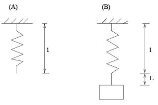
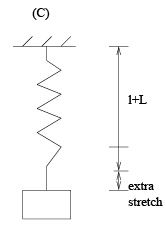
Figure (A): a spring in rest, with length l.
Figure (B): we put a mass m on the spring, and the spring is stretched. We call length L the elongation.
Figure (C): The spring-mass system is set in motion by stretch/squueze it extra, with initial velocity, or with external force.
Force diagram at equilibrium position: mg = F s.
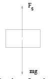
Hooke’s law: Spring force Fs = −kL, where L =elongation and k =spring constant.
So: we have mg = kL which give

which gives a way to obtain k by experiment: hang a mass m and measure the elongation L.
Model the motion: Let u(t) be the displacement/position of the mass at time t, assuming the origin u = 0 is at the equilibrium position, and downward is the positive direction.
Total elongation: L + u Total spring force: Fs = −k(L + u) Other forces:
- damping/resistent force:
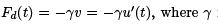 is the damping constant, and v is the velocity
 - External force applied on the mass: F (t), given function of t
Total force on the mass:
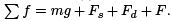
Newton’s law of motion ma =  gives
gives

Since mg = kL, by rearranging the terms, we get
mu′′ + γu′ + ku = F
where m ia the mass, γ is the damping constant, k is the spring constant, and F is the external force.
Next we study several cases.
Case 1: Undamped free vibration (simple harmonic motion). We assume no damping (γ = 0) and no external force (F = 0). So the equation becomes
mu′′ + ku = 0.
Solve it
General solution
u(t) = c1 cos ω0t + c2 sin ω0t.
Four terminologies of this motion: frequency, period, amplitude and phase, defined below.
Frequency: 
Period:
Amplitude and phase: We need to work on this a bit. We can write
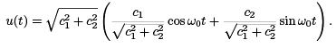
Now, define 
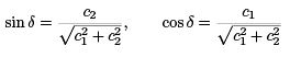
so we have
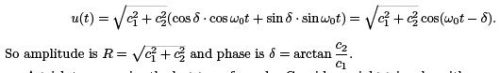
A trick to memorize the last term formula: Consider a right triangle, with c1 and c2 as the sides that form the right angle. Then, the amplitude equals to the length of the hypotenuse, and the phase δ is the angle between side c1 and the hypotenuse. Draw a graph and you will see it better.
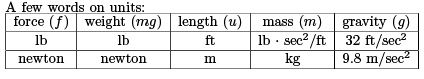
Problems in this part often come in the form of word problems. We need to learn the skill of extracting information from the text and put them into mathematical terms.
Example 1. A mass weighing 10 lb stretches a spring 2 in. We neglect damping. If the mass is displaced an additional 2 in, and is then set in motion with initial upward velocity of 1 ft/sec, determine the position, frequency, period, amplitude and phase of the motion.
Answer.We see this is free harmonic oscillation. The equation is
mu′′ + ku = 0
with initial conditions (Pay attention to units!)
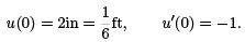
We need find the values for m and k. We have
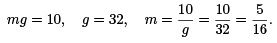
To find k, we see that the elongation is 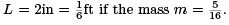 By Hooke’s law, we have
kL = mg, k = mg/L = 60.
Put in these values, we get the equation
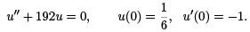
So the frequency is  and the general solution is
u(t) = c1 cos ω0t + c2 sin ω0t
We can find c1 , c2 by the ICs:
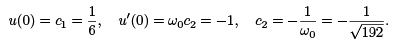
(Note that c1 = u(0) and c2 = u′ (0)/ω0 .) Now we have the position at any time t
The four terms of the motion are
and

Case II: Damped free vibration. We assume that γ ≠ 0(> 0) and F = 0.
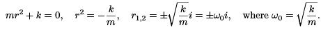
mu′′ + γ u′ + ku = 0
then
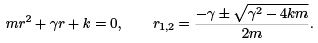
We see the type of root depends on the sign of the discriminant  − 4km.
- If
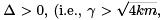 large damping,) we have two real roots, and they are both negative. The general solution is
Due to the large damping force, there will be no vibration in the motion. The mass will simply return to the equilibrium position exponentially. This kind of motion is called overdamped. - If
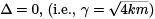 we have double roots r1 = r2 = r < 0. So u = (c1 + c2 t)ert .
Depending on the sign of c1 , c2 (which is determined by the ICs), the mass may cross the equilibrium point maximum once. This kind of motion is called critically damped, and this value of γ is called critical damping. - If
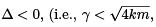 small damping) we have complex roots
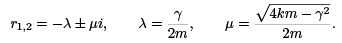
So the position function is
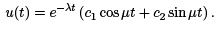
This motion is called damped oscillation. We can re-write it as
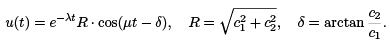
Here the term e−λt R is the amplitude, and µ is called the quasi frequency, and the quasi period is  The graph of the solution looks like the one for complex roots with negative real part.
Summary: For all cases, since the real part of the roots are always negative, u will go to zero as t grow. This means, if there is damping, no matter how big or small, the motion will eventually come to a rest.
Example 2. A mass of 1 kg is hanging on a spring with k = 1. The mass is in a medium that exerts a viscous resistance of 6 newton when the mass has a velocity of 48 m/sec. The mass is then further stretched for another 2m, then released from rest. Find the position u(t) of the mass.
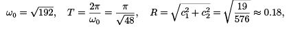
Answer. We have  So the equation for u is

Solve it
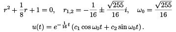
By ICs, we have u(0) = c1 = 2, and
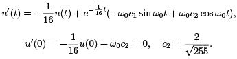
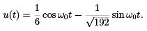
So the position at any time t is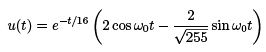
Forced Vibrations
In this chapter we assume the external force is F (t) = F0 cos ωt. (The case where F (t) = F0 sin ωt is totally similar.) The reason for this particular choice of force will be clear later when we learn Fourier series, i.e., we represent periodic functions with the sum of a family of sin and cos functions.
Case 1: With damping.
mu′′ + γ u′ + ku = F0 cos ωt.
Solution consists of two parts:
u(t) = uH (t) + U (t), uH (t): the solution of the homogeneous equation, U (t): a particular solution for the non-homogeneous equation.
From discussion is the previous chapter, we know that uH → 0 as t → +∞ for systems with damping. Therefore, this part of the solution is called the transient solution.
The appearance of U is due to the force term F . Therefore it is called the forced response.
The form of this particular solution is U (t) = A1 cos ωt + A2 sin ωt. As we have seen, we can rewrite it as U (t) = R cos(ωt − δ) where R is the amplitude and δ is the phase.
We see it is a periodic oscillation for all time t.
As time t → ∞, we have u(t) → U (t). So U (t) is called the steady state.
Case 2: Without damping. The equation now is
mu′′ + ku = F0 cos ωt
Let w0 =  denote the system frequency (i.e., the frequency for the free oscillation). The homogeneous solution is
uH (t) = c1 cos ω0t + c2 sin ω0t.
The form of the particular solution depends on the value of w. We have two cases.
Case 2A: if w ≠ w0 . The particular solution is of the form
U = A cos wt.
(Note that we did not take the sin wt term, because there is no u′ term in the equation.) And U ′′ = −w2A cos wt. Plug these in the equation
m(−w2A cos wt) + kA cos wt = F0 cos wt,

Note that if w is close to w0 , then A takes a large value.
General solution u(t) = c1 cos w0 t + c2 sin w0t + A cos wt where c1 , c2 will be determined by ICs.
Now, assume ICs:
u(0) = 0, u′(0) = 0.
Let’s find c1 , c2 and the solution:
u(0) = 0 : c1 + A = 0, c1 = −A u′ (0) = 0 : 0 + w0c2 + 0 = 0, c2 = 0
Solution
u(t) = −A cos w0t + A cos wt = A(cos wt − cos w0t).
We see that the solution consists of the sum of two cosine functions, with different frequencies. In order to have a better idea of how the solution looks like, we apply some manipulation.
Recall the trig identity:
We now have
Since both w0 , w are positive, then w0 + w has larger value than w0 − w. Then, the first term  can be viewed as the varying amplitude, and the second term
 is the vibration/oscillation.
One particular situation of interests: if w0 ≠ w but they are very close wo ≈ w, then we have |w0 − w| << |w0 + w|, meaning that |w0 − w| is much smaller than |w0 + w|. The plot of u(t) looks like (we choose w0 = 9, w = 10)
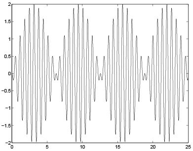
This is called a beat. (One observes it by hitting a key on a piano that’s not tuned, for example.)
Case 2B: If w = w0 . The particular solution is U = At cos w0t + B t sin w0t
A typical plot looks like:
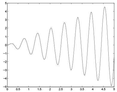
This is called resonance. If the frequency of the source term ω equals to the frequency of the system ω0, then, small source term could make the solution grow very large!
One can bring down a building or bridge by small periodic perturbations.
Historical disasters such as the French troop marching over a bridge and the bridge collapsed. Why? Unfortunate for the French, the system frequency of the bridge matches the frequency of their foot-steps.
FAQs on Linear Ordinary Differential Equations of First and Second Order - 6 - Physics for IIT JAM, UGC - NET, CSIR NET
| 1. What is a linear ordinary differential equation (ODE) of first order? |  |
| 2. How do you solve a first-order linear ODE? | |
| 3. What is a linear ordinary differential equation (ODE) of second order? | |
| 4. How do you solve a second-order linear ODE? | |
| 5. How are linear ODEs used in physics? | |


Important questions
,Previous Year Questions with Solutions
,shortcuts and tricks
,Extra Questions
,Semester Notes
,Linear Ordinary Differential Equations of First and Second Order - 6 | Physics for IIT JAM
,Summary
,CSIR NET
,ppt
,UGC - NET
,CSIR NET
,Linear Ordinary Differential Equations of First and Second Order - 6 | Physics for IIT JAM
,study material
,UGC - NET
,Viva Questions
,UGC - NET
,practice quizzes
,MCQs
,Sample Paper
,Objective type Questions
,mock tests for examination
,Linear Ordinary Differential Equations of First and Second Order - 6 | Physics for IIT JAM
,Exam
,past year papers
,Free
,CSIR NET
,video lectures
,


Linear Ordinary Differential Equations of First and Second Order - 6 Free PDF Download
Importance of Linear Ordinary Differential Equations of First and Second Order - 6
Linear Ordinary Differential Equations of First and Second Order - 6 Notes
Linear Ordinary Differential Equations of First and Second Order - 6 Physics Questions
Study Linear Ordinary Differential Equations of First and Second Order - 6 on the App
|
© EduRev
|
Education Revolution
|


|


within 7 days!