Analytic Functions - 2 | Physics for IIT JAM, UGC - NET, CSIR NET PDF Download

3. Analogous Situations in Physics. We shall not go farther back than Newton in tracing the development in mathematical physics. With the name of Newton we associate a great many things, but here we are interested in particular in two. First, in the general laws of mechanics stating that the time rate of change of the momentum is equal to force
(23)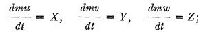
and, second, in the special case (inverse square law) in which the force components are given by
(24) 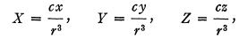
which should be compared with (3). We have here the attracting point, and the attracted point, both as discrete points. One of the trends of physics has been the transition from the consideration of discrete points to the consideration of fields, that is, continuously distributed quantities. We shall follow this trend separately for the right-hand sides and the left-hand sides of the equations, that is, the forces and matter.
First, as to the forces, we find easily that the force components given by the explicit formulas (24) satisfy the differential equations
(25) 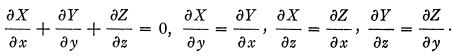
This is at the same time a generalization of the inverse square law and its source. We can get the inverse square law back from these differential equations by solving them under the additional condition of symmetry around a point. In passing from an explicit expression for the law of force to the partial differential equations we shifted our attention, without changing any essential features of the situation, from the singularities of the field to the field connected with these singularities.
We may do a similar thing to the left-hand sides of our equations, and introduce a continuous fluid instead of a discrete particle (the case of a particle may then be obtained as a limiting case of infinite density). Mathematically, this transition is a transition from ordinary to partial differential equations. In the simplest case, that of steady motion, when density is constant, and there exists a potential of velocities, the equations satisfied by the components of velocity are
(26) 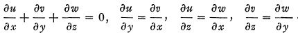
These equations were known in the 18th century; they appear for instance, in a memoir of Lagrange* in 1760; the remarkable thing is that these equations of the simplest motion of a fluid are the same as those of the simplest field of force. Furthermore these equations are exactly the case n = 3 of the Volterra theory (§2) and thus a generalization of the equations (1) of the theory of analytic functions. The inverse square law appears as the simplest singularity corresponding to w = c/z (compare formulas (3) and (24)) ; the exponent in the denominator is equal to the number of dimensions in each case. The residue corresponds to the mass, or electric charge of the attracting point.
In considering cases more general than the simple one just mentioned the ways of the forces and those of the velocities part , a t least for a time. For hydrodynamic s we hav e to use in th e general case th e equations of Euler, which we tak e in th e following form :
(27) 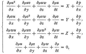
where p is th e pressure an d p is th e density. Th e first three of these equation s correspond to th e three equation s (23), and are nothin g bu t their translation into th e language of continuous distribution ; th e last one is a translatio n of th e equatio n dm/dt = Of which is usually no t writte n ou t explicitly in th e discrete case.
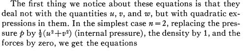
(28)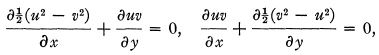
which are exactly th e equation s (7) for wha t we hav e called W in th e theor y of analyti c functions. Wit h th e same assumptions, bu t for n = 3, we get
(29) 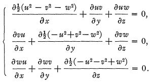
We naturally ask about the relation between these differential equations for the quadratic quantities and the differential equations written out before for the linear quantities. As in the case n = 2, the equations for the second-degree quantities are consequences of those for the linear quantities, but in contradistinction from that case we cannot pass here from (29) to (26) ; this raises the question : what additional conditions have to be imposed on the quadratic quantities so that the linear equations would be satisfied ?
The form of Euler's set of equations suggests the consideration of the case n = 4, by considering time as the fourth coordinate and / as the fourth component of the vector (u, vy w, f). Taking this suggestion seriously means making the first step toward the special theory of relativity. Without entering into details we must mention that velocity is represented in this theory by a four-vector, whose components we may denote by uir and that if we consider from this point of view matter in the absence of forces, we arrive at a set of equations which constitute the generalization for four dimensions of (28) and (29).
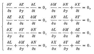
We shall now return to the consideration of forces. We spoke of the inverse square law without mentioning the physical nature of the forces. Historically, the gravitational field was the one for which in the time of Newton the inverse square law was formulated. But we are now more interested in the electrostatic and magnetostatic fields to which the same law has been applied in the nineteenth century. To each of these fields taken separately that law, and therefore the equation (25), applies. As soon as the time is introduced, however, that is, as soon as we begin to consider fields changing with time, interaction between these fields appears, and we have to consider them together. The result may be formulated as follows. In the static case the quantities δY/δz-δZ/δy, δZ/δx-δX/δz, δX/δy-δY/δx and δM/δz — δN/δy, δN/δx — δL/δz, dL/δy — δM/δx were zero. For the case when the fields change with time, Faraday's discoveries coupled with Maxwell's imagination resulted in equating these quantities (I omit the factor of proportionality), respectively, to δL/δt, δM/δt, δN/δt and -δX/δt, -δY/δt, -δZ/δt, so that together with the equations expressing the vanishing of the divergences we have the following set of equations for electromagnetic forces in matter-free space (Maxwell's equations) :
(30) 
It seems surprising now that until 1907 it was not noticed that the best way to write these equations was the four-dimensional way already suggested by the form of Euler's equations (27). The explanation is that the equations were encumbered with matter and three-dimensional vector analysis. Moreover, the really fundamental things have a way of appearing to be simple once they have been stated by a genius, who was in this case Minkowski.
Another thing is almost as remarkable—the equations at which we have arrived are, except for some differences in sign, th e sam e a s th e equation s (20) of th e Volterr a theor y for n=4 , r = 2. It remained for L. Hanni* to notice this fact in 1910. We have thus again in mathematical physics a generalization of the theory of analytic functions. The difference in sign is of extreme importance in physics. It may be stated that without this difference our world would have been dark; the minus sign that appears in the above quantities makes light possible. In this connection we might mention that if we eliminate all dependent functions but one from Maxwell's equations, we obtain, due to this difference in sign, instead of the Laplace equation that appears as a result of such elimination in the cases considered above, an equation of the type
(31) 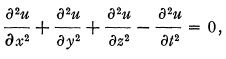
which differs from the Laplace equation by the minus sign before the last term. This is the so called wave equation; it received its name from the fact that it is often used in describing wave phenomena, especially in acoustics, and in optics in connection with what is called the wave theory of light. From the mathematical point of view the introduction by Maxwell of the electromagnetic theory of light may be considered as essentially the substitution for a theory based on one second-order partial differential equation of a theory based on a. system of first-order equations (of which the second-order equation is a consequence). We want to emphasize this fact in view of an analogous situation to be mentioned later. We may mention also the fact that the main importance of this substitution seems to lie in its effect in introducing boundary conditions.
The lack of beauty due to the difference in sign may be remedied by the introduction of slight modifications in our notations. If we use instead of (21), the notations
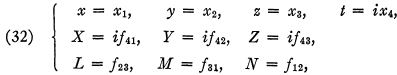
and instead of (19) the relations
(33) 
the equations of Maxwell assume exactly the form (20). The introduction of these notations constitutes the second step toward the special theory of relativity.
4. Second-Degree Quantities in Electrodynamics. : We noticed before that in Euler's hydrodynamic equations (27) the quantities u, v, w appear not directly, but as certain quadratic combinations; in the two- and three-dimensional cases written out above (28) and (29) the quantities subjected to differentiation are the elements of the matrices
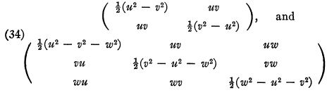
The differential equations (28) and (29) may be expressed by stating that the divergences of these matrices vanish. In fourspace (special relativity theory) there also appears a matrix of the same nature which we write out in index notation:
(35) 
In the electromagnetic theory analogous combinations of force components were introduced by Maxwell under the name of stress components. When we treat, in three-dimensional space, electric and magnetic forces separately, the stresses are
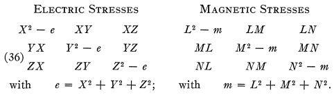
We may note that if we impose on the forces the equations (25), the divergence of the stress matrix vanishes, but we shall return to the question of differential relations later. We saw that the electric and magnetic forces are interrelated, and that the situation is best expressed in four-dimensional notations. Therefore there seems to be no reason for keeping the electric and magnetic stresses apart, and so we combine the above matrices by simply adding the corresponding elements together. We extend the three-rowed matrix thus obtained into a four-rowed matrix by adding a fourth row and a fourth column. We shall not write out this four-rowed matrix in full, nor shall we explain the physical meaning (which is a very important one) of the new additional quantities. Instead we shall write it in short notations which will bring out even more clearly the relation to the theory of analytic functions. We have here two surface vectors ƒ and r represented by four-rowed matrices as our first-degree quantities. In terms of them, the four-rowed matrix of the stresses is
(37) 
or, in index notation,
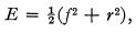
(38) 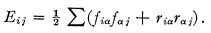
Here/2 and r2 may be considered as matrices obtained from the matrices ƒ and r by squaring them in the manner employed in squaring a determinant. The expression obtained is a matrix which depends quadratically on the force matrix. The relation between the force matrices ƒ and r on the one hand, and the matrix E on the other is analogous to the relation between the first-degree and the second-degree quantities in the theory of analytic functions. In some ways it reminds us of the quantity W. It is, like W, a matrix, and the analogy between W and E guided us in the formation of E, especially in the three-dimensional stage. As a finished product, however, E resembles more Q. In the first place, it possesses the same form (compare formulas (6)) ; in the second place, the relationship between E and Q appears very clearly when we ask ourselves whether the forces given by ƒ are determined when E is given. Just as in the case of analytic functions, if (X, F, Z) and (L, M, N) produce certain stresses, the quantities
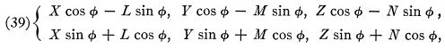
where φ is an arbitrary function of x, y, z> and /, produce the same stresses. These formulas are analogous to (9).
We pass now to the consideration of differential equations satisfied by the stresses. The matrix E, as was the case with W in the case of an analytic function, satisfies, as a result of (ƒ, r) satisfying Maxwell's equations, a set of linear differential equations which may be written in the form
(40) 
and is strictly analogous to equations (7). This analogy appears more clearly when the last equations are written out in components. But these equations do not constitute a sufficient condition for a stress matrix to be derived from forces which satisfy Maxwell's equations. Subjecting to Maxwell's equations (30) the above expressions (39) for the forces corresponding to a given stress matrix, we obtain a set of eight equations on the derivatives of the heretofore arbitrary angle φ. The vanishing of the divergence of E (see equations (40)) is exactly the set of conditions for algebraic compatibility of these equations. In addition to that, however, certain integ?'ability conditions must be satisfied. They furnish another non-linear set of differential equations for E. We shall not write out these equations,* but for the purpose of further reference we shall put down the equations on the derivatives of the angle φ, which (derivatives) we shall denote by φ1, φ2, φ3, φ4 '
(41) 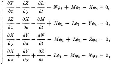
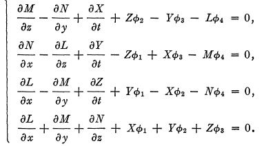
These equations are the analogs of (10).
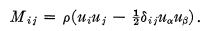
In what precedes we have treated separately the components of the forces and the components of matter corresponding to the right hand sides and the left hand sides of the original equations of motion (23). Although in the description of the further fate of these quantities the theory of analytic functions—our guiding light—ceases to play a leading role, we do not want to abandon forces and matter without mentioning that they become happily reunited by simply adding together the corresponding elements of the matrices Mij (35) and Eij (38) into the elements of a matrix Tij , and that the equations of motion may then be written simply by saying that the divergence of this new matrix is zero. The new equations of motion differ slightly from the old ones but seem to be in keeping with experiments. At this point another of the theories of pure mathematics becomes of extreme importance, namely, the theory of surfaces together with its generalization, the theory of curved spaces (riemannian geometry). A discussion of the interrelation between these two theories of pure mathematics, and also the application of the second to physics, space does not permit to take up here. It will suffice to say that the identification of the matrix Tij with a tensor appearing in the theory of curved spaces leads to the general relativity theory,
FAQs on Analytic Functions - 2 - Physics for IIT JAM, UGC - NET, CSIR NET
| 1. What are analytic functions in physics? |  |
| 2. How are analytic functions applied in physics? | |
| 3. What is the significance of analytic functions in physics? | |
| 4. Can non-analytic functions be used to describe physical phenomena? | |
| 5. Are there any limitations to the use of analytic functions in physics? | |


Semester Notes
,CSIR NET
,Free
,ppt
,mock tests for examination
,Extra Questions
,Previous Year Questions with Solutions
,CSIR NET
,Analytic Functions - 2 | Physics for IIT JAM
,UGC - NET
,Important questions
,past year papers
,shortcuts and tricks
,Sample Paper
,CSIR NET
,Summary
,practice quizzes
,Analytic Functions - 2 | Physics for IIT JAM
,UGC - NET
,Objective type Questions
,Analytic Functions - 2 | Physics for IIT JAM
,MCQs
,study material
,Viva Questions
,video lectures
,Exam
,UGC - NET
;


Analytic Functions - 2 Free PDF Download
Importance of Analytic Functions - 2
Analytic Functions - 2 Notes
Analytic Functions - 2 Physics Questions
Study Analytic Functions - 2 on the App
|
© EduRev
|
Education Revolution
|


|


within 7 days!