Random Variables:Discrete and Continuous - Mathematical Methods of Physics, UGC - NET Physics | Physics for IIT JAM, UGC - NET, CSIR NET PDF Download

A random variable, usually written X, is a variable whose possible values are numerical outcomes of a random phenomenon. There are two types of random variables, discrete and continuous.
Discrete Random Variables
A discrete random variable is one which may take on only a countable number of distinct values such as 0,1,2,3,4,........ Discrete random variables are usually (but not necessarily) counts. If a random variable can take only a finite number of distinct values, then it must be discrete. Examples of discrete random variables include the number of children in a family, the Friday night attendance at a cinema, the number of patients in a doctor's surgery, the number of defective light bulbs in a box of ten.
The probability distribution of a discrete random variable is a list of probabilities associated with each of its possible values. It is also sometimes called the probability function or the probability mass function.
Suppose a random variable X may take k different values, with the probability that X = xi defined to be P(X = xi) = pi. The probabilities pi must satisfy the following:
1: 0 < pi < 1 for each i
2: p1 + p2 + ... + pk = 1.
Example
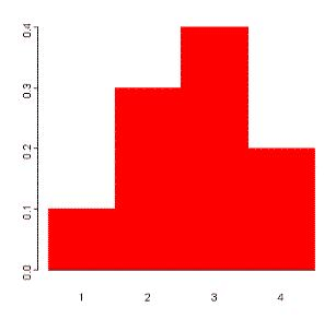
Suppose a variable X can take the values 1, 2, 3, or 4.
The probabilities associated with each outcome are described by the following table:
Outcome 1 2 3 4
Probability 0.1 0.3 0.4 0.2
The probability that X is equal to 2 or 3 is the sum of the two probabilities: P(X = 2 or X = 3) = P(X = 2) + P(X = 3) = 0.3 + 0.4 = 0.7. Similarly, the probability that X is greater than 1 is equal to 1 - P(X = 1) = 1 - 0.1 = 0.9, by the complement rule.
This distribution may also be described by the probability histogram shown to the right:
All random variables (discrete and continuous) have a cumulative distribution function. It is a function giving the probability that the random variable X is less than or equal to x, for every value x. For a discrete random variable, the cumulative distribution function is found by summing up the probabilities.
Example
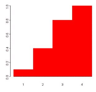
The cumulative distribution function for the above probability distribution is calculated as follows:
The probability that X is less than or equal to 1 is 0.1,
the probability that X is less than or equal to 2 is 0.1+0.3 = 0.4,
the probability that X is less than or equal to 3 is 0.1+0.3+0.4 = 0.8, and
the probability that X is less than or equal to 4 is 0.1+0.3+0.4+0.2 = 1.
The probability histogram for the cumulative distribution of this random variable is shown to the right:
Continuous Random Variables
A continuous random variable is one which takes an infinite number of possible values. Continuous random variables are usually measurements. Examples include height, weight, the amount of sugar in an orange, the time required to run a mile.
A continuous random variable is not defined at specific values. Instead, it is defined over an interval of values, and is represented by the area under a curve (in advanced mathematics, this is known as an integral). The probability of observing any single value is equal to 0, since the number of values which may be assumed by the random variable is infinite.
Suppose a random variable X may take all values over an interval of real numbers. Then the probability that X is in the set of outcomes A, P(A), is defined to be the area above A and under a curve. The curve, which represents a function p(x), must satisfy the following:
1: The curve has no negative values (p(x) > 0 for all x)
2: The total area under the curve is equal to 1.
A curve meeting these requirements is known as a density curve.
The Uniform Distribution
A random number generator acting over an interval of numbers (a,b) has a continuous distribution. Since any interval of numbers of equal width has an equal probability of being observed, the curve describing the distribution is a rectangle, with constant height across the interval and 0 height elsewhere. Since the area under the curve must be equal to 1, the length of the interval determines the height of the curve.
The following graphs plot the density curves for random number generators over the intervals (4,5) (top left), (2,6) (top right), (5,5.5) (lower left), and (3,5) (lower right). The distributions corresponding to these curves are known as uniform distributions.
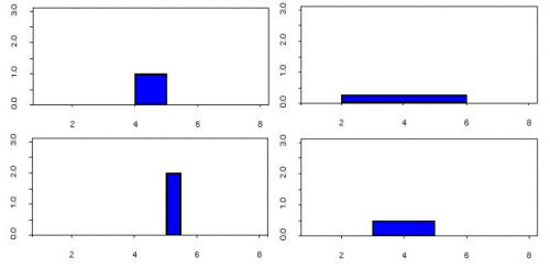
Consider the uniform random variable X defined on the interval (2,6). Since the interval has width = 4, the curve has height = 0.25 over the interval and 0 elsewhere. The probability that X is less than or equal to 5 is the area between 2 and 5, or (5-2)*0.25 = 0.75. The probability that X is greater than 3 but less than 4 is the area between 3 and 4, (4-3)*0.25 = 0.25. To find that probability that X is less than 3 orgreater than 5, add the two probabilities:
P(X < 3 and X > 5) = P(X < 3) + P(X > 5) = (3-2)*0.25 + (6-5)*0.25 = 0.25 + 0.25 = 0.5.
The uniform distribution is often used to simulate data. Suppose you would like to simulate data for 10 rolls of a regular 6-sided die. Using the MINITAB "RAND" command with the "UNIF" subcommand generates 10 numbers in the interval (0,6):
MTB > RAND 10 c2;
SUBC> unif 0 6.
Assign the discrete random variable X to the values 1, 2, 3, 4, 5, or 6 as follows:
if 0<X<1, X=1
if 1<X<2, X=2
if 2<X<3, X=3
if 3<X<4, X=4
if 4<X<5, X=5
if X>5, X=6.
Use the generated MINITAB data to assign X to a value for each roll of the die:
Uniform Data X Value
4.53786 5
5.77474 6
3.69518 4
1.03929 2
4.23835 5
0.37096 1
0.75272 1
5.56563 6
0.89045 1
3.18086 4
Another type of continuous density curve is the normal distribution. The area under the curve is not easy to calculate for a normal random variable X with mean μ and standard deviation σ. However, tables (and computer functions) are available for the standard random variable Z, which is computed from X by subtracting μ and dividing by σ. All of the rules of probability apply to the normal distribution.
FAQs on Random Variables:Discrete and Continuous - Mathematical Methods of Physics, UGC - NET Physics - Physics for IIT JAM, UGC - NET, CSIR NET
| 1. What is the difference between discrete and continuous random variables? |  |
| 2. How do we determine the probability distribution of a discrete random variable? | |
| 3. Can a random variable be both discrete and continuous? | |
| 4. What are some examples of discrete random variables in physics? | |
| 5. What are some examples of continuous random variables in physics? | |


Objective type Questions
,UGC - NET
,Semester Notes
,practice quizzes
,mock tests for examination
,MCQs
,ppt
,CSIR NET
,UGC - NET
,Extra Questions
,UGC - NET Physics | Physics for IIT JAM
,Exam
,Random Variables:Discrete and Continuous - Mathematical Methods of Physics
,Important questions
,Summary
,UGC - NET
,past year papers
,Free
,Random Variables:Discrete and Continuous - Mathematical Methods of Physics
,shortcuts and tricks
,study material
,Viva Questions
,UGC - NET Physics | Physics for IIT JAM
,CSIR NET
,CSIR NET
,video lectures
,Sample Paper
,Random Variables:Discrete and Continuous - Mathematical Methods of Physics
,UGC - NET Physics | Physics for IIT JAM
,Previous Year Questions with Solutions
;


Random Variables:Discrete and Continuous - Mathematical Methods of Physics, UGC - NET Physics Free PDF Download
Importance of Random Variables:Discrete and Continuous - Mathematical Methods of Physics, UGC - NET Physics
Random Variables:Discrete and Continuous - Mathematical Methods of Physics, UGC - NET Physics Notes
Random Variables:Discrete and Continuous - Mathematical Methods of Physics, UGC - NET Physics Physics Questions
Study Random Variables:Discrete and Continuous - Mathematical Methods of Physics, UGC - NET Physics on the App
|
© EduRev
|
Education Revolution
|


|


