Finite Differences - Numerical Analysis, CSIR-NET Mathematical Sciences | Mathematics for IIT JAM, GATE, CSIR NET, UGC NET PDF Download

Finite Difference Methods for Partial Differential Equations
As you are well aware, most differential equations are much too complicated to be solved by an explicit analytic formula. Thus, the development of accurate numerical approximation schemes is essential for both extracting quantitative information as well as achieving a qualitative understanding of the behavior of their solutions. Even in cases, such as the heat and wave equations, where explicit solution formulas (either closed form or infinite series) exist, numerical methods still can be profitably employed. Indeed, the lessons learned in the design of numerical algorithms for “solved” examples are of inestimable value when confronting more challenging problems. Furthermore, one has the ability to accurately test a proposed numerical algorithm by running it on a known solution.
Basic numerical solution schemes for partial differential equations fall into two broad categories. The first are the finite difference methods , obtained by replacing the derivatives in the equation by the appropriate numerical differentiation formulae. However, there is no guarantee that the resulting numerical scheme will accurately approximate the true solution, and further analysis is required to elicit bona fide, convergent numerical algorithms.
We thus start with a brief discussion of simple finite difference formulae for numerically approximating low order derivatives of functions. The ensuing sections establish some of the most basic finite difference schemes for the heat equation, first order transport equations, and the second order wave equation. As we will see, not all finite difference approximations lead to accurate numerical schemes, and the issues of stability and convergence must be dealt with in order to distinguish valid from worthless methods. In fact, inspired by Fourier analysis, the basic stability criterion for a finite difference scheme is based on how the scheme handles complex exponentials.
We will only introduce the most basic algorithms, leaving more sophisticated variations and extensions to a more thorough treatment, which can be found in numerical analysis texts, e.g., [ 5, 7, 29 ].
11.1. Finite Differences.
In general, to approximate the derivative of a function at a point, say f ′(x) or f ′′(x), one constructs a suitable combination of sampled function values at nearby points. The underlying formalism used to construct these approximation formulae is known as the calculus of finite differences . Its development has a long and influential history, dating back to Newton. The resulting finite difference numerical methods for solving differential equations have extremely broad applicability, and can, with proper care, be adapted to most problems that arise in mathematics and its many applications.
The simplest finite difference approximation is the ordinary difference quotient
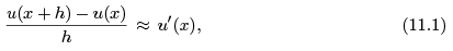
used to approximate the first derivative of the function u(x). Indeed, if u is differentiable at x, then u′ (x) is, by definition, the limit, as h → 0 of the finite difference quotients.
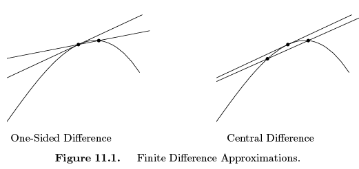
Throughout our discussion, h, the step size , which may be either positive or negative, is assumed to be small: | h | << 1. When h > 0, (11.1) is referred to as a forward difference , while h < 0 gives a backward difference . Geometrically, the difference quotient equals the slope of the secant line through the two points  on the graph of the function. For small h, this should be a reasonably good approximation to the slope of the tangent line, u′ (x), as illustrated in the first picture in Figure 11.1.
How close an approximation is the difference quotient? To answer this question, we assume that u(x) is at least twice continuously differentiable, and examine the first order Taylor expansion

We have used the Cauchy form for the remainder term, [ 2], in which ξ represents some point lying between x and x + h. The error or difference between the finite difference formula and the derivative being approximated is given by

Since the error is proportional to h, we say that the finite difference quotient (11.3) is a first order approximation. When the precise formula for the error is not so important, we will write

The “big Oh” notation O(h) refers to a term that is proportional to h, or, more rigorously, bounded by a constant multiple of h as h → 0.
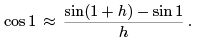
Example 11.1. Let u(x) = sin x. Let us try to approximate u′ (1) = cos 1 = .5403023 . . . by computing finite difference quotients
The result for different values of h is listed in the following table.
| h | 1 | .1 | .01 | .001 | .0001 |
| approximation | .067826 | .497364 | .536086 | .539881 | .540260 |
| error | −.472476 | −.042939 | −.004216 | −.000421 | −.000042 |
We observe that reducing the step size by a factor of 110 reduces the size of the error by approximately the same factor. Thus, to obtain 10 decimal digits of accuracy, we anticipate needing a step size of about h = 10−11 . The fact that the error is more of less proportional to the step size confirms that we are dealing with a first order numerical approximation.
To approximate higher order derivatives, we need to evaluate the function at more than two points. In general, an approximation to the nth order derivative u(n) (x) requires at least n + 1 distinct sample points. For simplicity, we shall only use equally spaced points, leaving the general case to the exercises.
For example, let us try to approximate u′′ (x) by sampling u at the particular points x, x + h and x − h. Which combination of the function values u(x − h), u(x), u(x + h) should be used? The answer to such a question can be found by consideration of the relevant Taylor expansions
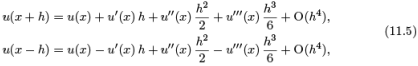
where the error terms are proportional to h4 . Adding the two formulae together gives
u(x + h) + u(x − h) = 2 u(x) + u′′(x) h2 + O(h4).
Rearranging terms, we conclude that

The result is known as the centered finite difference approximation to the second derivative of a function. Since the error is proportional to h2 , this is a second order approximation.
Example 11.2. Let us approximate u′′ (1) = 6 e = 16.30969097 . . . by using the finite difference quotient (11.6):
The results are listed in the following table.
| h | 1 | .1 | .01 | .001 | .0001 |
| approximation | 5.16158638 | 16.48289823 | 16.31141265 | 16.30970819 | 16.30969115 |
| error | 33.85189541 | .17320726 | .00172168 | .00001722 | .00000018 |
Each reduction in step size by a factor of 110 reduces the size of the error by a factor of 1/100 and results in a gain of two new decimal digits of accuracy, confirming that the finite difference approximation is of second order.
However, this prediction is not completely borne out in practice. If we take† h = .00001 then the formula produces the approximation 16.3097002570, with an error of .0000092863 — which is less accurate that the approximation with h = .0001. The problem is that round-off errors have now begun to affect the computation, and underscores the difficulty with numerical differentiation. Finite difference formulae involve dividing very small quantities, which can induce large numerical errors due to round-off. As a result, while they typically produce reasonably good approximations to the derivatives for moderately small step sizes, to achieve high accuracy, one must switch to a higher precision. In fact, a similar comment applied to the previous Example 11.1, and our expectations about the error were not, in fact, fully justified as you may have discovered if you tried an extremely small step size.
Another way to improve the order of accuracy of finite difference approximations is to employ more sample points. For instance, if the first order approximation (11.4) to the first derivative based on the two points x and x + h is not sufficiently accurate, one can try combining the function values at three points x, x + h and x − h. To find the appropriate combination of u(x − h), u(x), u(x + h), we return to the Taylor expansions (11.5). To solve for u′ (x), we subtract‡ the two formulae, and so
Rearranging the terms, we are led to the well-known centered difference formula
which is a second order approximation to the first derivative. Geometrically, the centered difference quotient represents the slope of the secant line through the two points  on the graph of u centered symmetrically about the point x. Figure 11.1 illustrates the two approximations; the advantages in accuracy in the centered difference version are graphically evident. Higher order approximations can be found by evaluating the function at yet more sample points, including, say, x + 2h, x − 2h, etc.
|
558 videos|198 docs
|
FAQs on Finite Differences - Numerical Analysis, CSIR-NET Mathematical Sciences - Mathematics for IIT JAM, GATE, CSIR NET, UGC NET
| 1. What is Finite Differences in numerical analysis? |  |
| 2. How does Finite Differences work in numerical analysis? | |
| 3. What are the advantages of using Finite Differences in numerical analysis? | |
| 4. What are the limitations of Finite Differences in numerical analysis? | |
| 5. How is Finite Differences used in solving differential equations? | |


shortcuts and tricks
,Viva Questions
,Finite Differences - Numerical Analysis
,GATE
,CSIR NET
,Important questions
,GATE
,mock tests for examination
,MCQs
,past year papers
,UGC NET
,CSIR-NET Mathematical Sciences | Mathematics for IIT JAM
,study material
,Sample Paper
,CSIR NET
,Exam
,Objective type Questions
,Semester Notes
,practice quizzes
,Extra Questions
,Summary
,CSIR-NET Mathematical Sciences | Mathematics for IIT JAM
,video lectures
,UGC NET
,GATE
,ppt
,UGC NET
,CSIR NET
,Finite Differences - Numerical Analysis
,Free
,Previous Year Questions with Solutions
,Finite Differences - Numerical Analysis
,CSIR-NET Mathematical Sciences | Mathematics for IIT JAM
;


Finite Differences - Numerical Analysis, CSIR-NET Mathematical Sciences Free PDF Download
Importance of Finite Differences - Numerical Analysis, CSIR-NET Mathematical Sciences
Finite Differences - Numerical Analysis, CSIR-NET Mathematical Sciences Notes
Finite Differences - Numerical Analysis, CSIR-NET Mathematical Sciences Mathematics Questions
Study Finite Differences - Numerical Analysis, CSIR-NET Mathematical Sciences on the App
|
© EduRev
|
Education Revolution
|


|


