Meaning and Types Of Markets- 2 | Business Economics for CA Foundation PDF Download
CONCEPTS OF TOTAL REVENUE, AVERAGE REVENUE AND MARGINAL REVENUE
Total Revenue: If a firm sells 100 units for ₹ 10 each, what is the amount which it realises? It realises ₹ 1,000 (100 x 10), which is nothing but the total revenue for the firm. Thus, we may state that total revenue or the total expenditure incurred by the purchasers of the firm’s product refers to the amount of money which a firm realises by selling certain units of a commodity. Symbolically, total revenue may be expressed as TR = P x Q
Where,
TR is total revenue
P is price
Q is quantity of a commodity sold
This may be represented by the following diagrams. In figure A, when the product of the price is ₹ 30, the quantity sold is 40 units. The total revenue is P x Q = ₹ 1200. Panel B shows the total revenue curve of a competitive firm having a perfectly elastic demand curve. Since the firm can sell any quantity at market determined prices, the TR curve is linear and starts from the origin. The TR curve of a firm which has a downward sloping demand curve is shown in figure 2.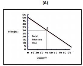
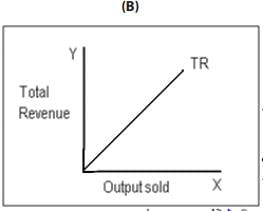
Figure 1: Total Revenue
Average Revenue: Average revenue is the revenue earned per unit of output. It is nothing but price of one unit of output because price is always per unit of a commodity. For this reason, average revenue curve is also the firms demand curve.
Symbolically, average revenue is:
Where
AR is average revenue
TR is the total revenue
Q is quantity of a commodity sold
If, for example, a firm realises total revenue of ₹ 1,000 by the sale of 100 units, it implies that the average revenue is ₹ 10 (1,000/100) or the firm has sold the commodity at a price of ₹ 10 per unit.
Marginal Revenue: Marginal revenue (MR) is the change in total revenue resulting from the sale of an additional unit of the commodity. Thus, if a seller realises ₹ 1,000 while selling 100 units and ₹ 1,200 while selling 101 units, we say that the marginal revenue is ` 200. We can say that MR is the rate of change in total revenue resulting from the sale of an additional unit of output 
Where
MR is marginal revenue
TR is total revenue
Q is quantity of a commodity sold
Δ stands for a small change
For one unit change in output
MRn = TRn – TRn-1
Where TR is the total revenue when sales are at the rate of n units per period.
TRn-1 is the total revenue when sales are at the rate of (n – 1) units per period.
In order to understand the above concepts clearly, look at Table -2. In column 1, the number of units sold of commodity X is given. Column 2 shows the total revenue fetched by selling different units. Column 3 shows average revenue which is nothing but price per unit. Column 4 shows marginal revenue which is addition to the total revenue by the sale of an additional unit of output.
Table 2: Total Revenue, Average Revenue and Marginal Revenue
Units | Total Revenue | Average Revenue | Marginal Revenue |
1 | 10 | 10 | 10 |
2 | 18 | 9 | 8 |
3 | 24 | 8 | 6 |
4 | 28 | 7 | 4 |
5 | 30 | 6 | 2 |
6 | 30 | 5 | 0 |
7 | 28 | 4 | -2 |
8 | 24 | 3 | -4 |
9 | 18 | 2 | -6 |
10 | 10 | 1 | -8 |
Note that the total revenue is maximum when 5 units of X are sold. It stays constant for one more unit and then begins to fall. Average revenue keeps on falling showing inverse relationship between price and quantity demanded. It represents demand function of X to the firm. Marginal revenue keeps on falling and after becoming zero it becomes negative. Also note that TR at any particular level of output is the sum of marginal revenues till that level of output.
The question which arises is: why is the marginal revenue due to the third unit (₹ 6) not equal to price of ` 8 at which the third unit is sold. The answer is that when price is reduced for selling an additional unit, the two units which could be sold for ₹ 9 before will have to be sold at the reduced price of ₹ 8 per unit. The total loss on previous two units due to price fall will be equal to ₹ 2. Thus, for any falling average revenue (or price) schedule, marginal revenue is always less than the price. In the case of constant average revenue (or price) schedule, the marginal revenue is equal to average revenue (or uniform price). If TR stands for total revenue and q stands for output, marginal revenue (MR) can be expressed as:
MR = dTR/dq
dTR/ dq indicates the slope of the total revenue curve.
When the demand curve of the firm is a normal downward sloping one, there is a well defined relationship between average revenue, marginal revenue and total revenue. This can be shown by the following figure presenting total revenue (TR), average revenue (AR) and marginal revenue (MR) curves. The average revenue curve in panel B is sloping downwards depicting the inverse relationship between price and quantity demanded. MR curve lies below AR curve showing that marginal revenue declines more rapidly than average revenue. Total revenue increases as long as marginal revenue is positive and declines (has a negative slope) when marginal revenue is negative. Total revenue curve initially increases at a diminishing rate due to diminishing marginal revenue and reaches maximum and then it falls. When marginal revenue becomes zero, the total revenue is maximum and the slope of TR is zero.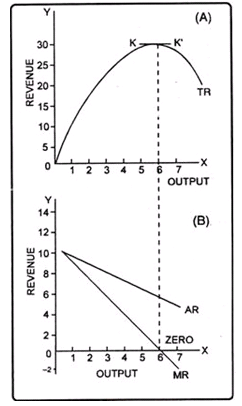
Fig. 2: Total Revenue, Average Revenue and Marginal Revenue Curves of a Firm which has downward Sloping Demand Curve
It may be noted that in all forms of imperfect competition, the average revenue curve of an individual firm slopes downwards as in these market forms, when a firm increases the price of its product, its quantity demanded decreases and vice versa. Under perfect competition, however, since the firms are price takers, the average revenue (or price) curve or demand curve is perfectly elastic. Perfectly elastic average revenue curve means that an individual firm has constant average revenue (or price). When price remains constant, marginal revenue will be equal to average revenue and thus AR curve and MR curve will coincide and will be horizontal curves as shown in figure 3. below.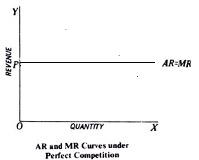
Fig 3: Average Revenue and Marginal Revenue Curves of a Perfectly Competitive Firm
RELATIONSHIP BETWEEN AR, MR, TR AND PRICE ELASTICITY OF DEMAND
It is to be noted that marginal revenue, average revenue and price elasticity of demand are uniquely related to one another through the formula: Where e = price elasticity of demand
and if e >1, MR will be positive
and if e <1, MR will be negative
In a straight line downward falling demand curve, we know that the coefficient of price elasticity at the middle point is equal to one. It follows that the marginal revenue corresponding to the middle point of the demand curve (or AR curve) will be zero. On the upper portion of the demand curve, where the elasticity is more than one, marginal revenue will be positive and on the lower portion of the demand curve where elasticity is less than one, marginal revenue will be negative. These can be shown in diagram :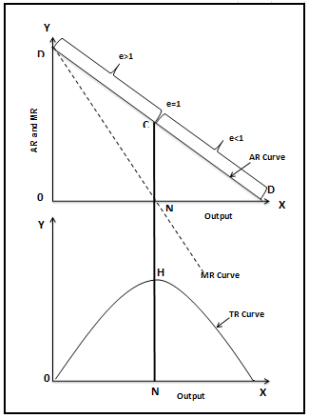
Fig.4: Relationship between AR, MR, TR and Price Elasticity of Demand
In fig. 4, DD is the AR or demand curve. At point C, elasticity is equal to one. Corresponding to C on the AR curve, the marginal revenue is zero. Thus, MR curve is touching X-axis at N (corresponding to C on the AR curve). At a greater quantity than ON, the elasticity of the AR curve is less than one and the marginal revenue is negative. Negative marginal revenue means MR curve goes below the X-axis to the fourth quadrant. Marginal revenue being negative means that total revenue will diminish if a quantity greater than ON is sold. Total revenue will be rising up to ON output since up to this the marginal revenue remains positive. It follows that total revenue will be maximum where elasticity is equal to one. Thus, TR is shown to be at its highest level at ON level of output (corresponding to the point C on AR curve). Beyond ON Level of output, the TR curve has a negative slope.
BEHAVIOURAL PRINCIPLES
Principle 1- A firm should not produce at all if its total variable costs are not met.
It is a matter of common sense that a firm should produce only if it will do better by producing than by not producing. The firm always has the option of not producing at all. If a firm’s total revenues are not enough to make good even the total variable costs, it is better for the firm to shut down. In other words, a competitive firm should shut down if the price is below AVC. In that case, it will minimise loss because then its total cost will be equal to its fixed costs and it will have an operating loss equal to its fixed cost. The sunk fixed cost is irrelevant to the shutdown decision because fixed costs are already incurred. This means that the minimum average variable cost is equal to the shut-down price, the price at which the firm ceases production in the short run. Shutting down is temporary and does not necessarily mean going out of business.
If price (AR) is greater than minimum AVC, but less than minimum ATC, the firm covers its variable cost and some but not all of fixed cost. If price is equal to minimum ATC, the firm covers both fixed and variable costs and earns normal profit or zero economic profit. If price is greater than minimum ATC, the firm not only covers its full cost, but also earns positive economic profit or super normal profit.
Principle 2 - The firm will be making maximum profits by expanding output to the level where marginal revenue is equal to marginal cost.
In other words, it will pay the firm to go on producing additional units of output so long as the marginal revenue exceeds marginal cost i.e., additional units add more to revenues than to cost. At the point of equality between marginal revenue and marginal cost, it will earn maximum profits.
The above principle can be better understood with the help of figure 5 which shows a set of hypothetical marginal revenue and marginal cost curves. Marginal revenue curve slopes downwards and marginal cost curve slopes upwards. They intersect each other at point E (MC= MR) which corresponds to output Q.* Up to Q* level of output, marginal revenue is greater than marginal cost and at output level *Q they are equal. The firm will be maximizing profits at E (or at Q* level of output). For all levels of output less than Q*, additional units of output add more to revenue than to cost (as their MR is more than MC) and thus it will be profitable for the firm to produce them. The firm will be foregoing profit equal to the area EFG if it stops at A. Similarly profits will fall, if a greater output than OQ is produced as they will add more to cost than to revenues. On the units from Qth to Bth, the firm will be incurring a loss equal to the area EHI.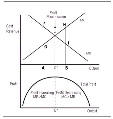
Fig: 5: Equilibrium of the Firm: Maximization of Profits
To conclude, the firm will maximize profits at the point at which marginal revenue is equal to marginal cost.
SUMMARY
|
|
86 videos|255 docs|58 tests
|
FAQs on Meaning and Types Of Markets- 2 - Business Economics for CA Foundation
| 1. What is the meaning of markets? |  |
| 2. What are the types of markets? |  |
| 3. How are prices determined in a market? |  |
| 4. What factors can affect the functioning of markets? |  |
| 5. How do markets contribute to economic growth? |  |

 Where e = price elasticity of demand .Total revenue will be maximum where elasticity is equal to one.


