Statistics and Probability (Part - 1) | Quantitative for GMAT PDF Download
Statistics
Fundamental Characteristics of Statistics
Statistics have the following important characteristics:
- Statistics are aggregate of facts and not a single observation.
- Statistics are expressed quantitatively.
- In an experiment statistics are related to each other and comparable. It can be classified into various groups.
- Statistics are collected for a pre-determined purpose.
- In collection of statistics a reasonable standard of accuracy must be maintained.
Limitations of Statistics
Statistics have the following limitations:
- Statistics is not fit for study of qualitative phenomenon like honesty, intelligence, poverty etc.
- Statistics deals with groups and does not study individuals.
- Laws of statistics are not exact. These are true on averages.
- Data collected for a definite purpose may not be suitable for another purpose.
Statistical Data
Statistical data are the facts which are collected for the purpose of investigation. There are two types of statistical data:
- Primary data: The data collected by an investigator for the first time for his own purpose are called primary data. As the primary data are collected by the user of the data, so it is more reliable and relevant.
- Secondary data: The data collected by a secondary source and used by the investigator for his purpose is called secondary data. For example score of a cricket match noted from newspapers is secondary data.
Thus data which are primary in the hands of one become secondary in the hands of the other.
Data collected by any source also can be divided in following two types:
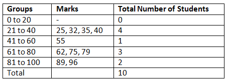
- Raw Data: Raw data are those data which are obtained from the original source but not arranged numerically. This is also called ‘ungrouped data’ for example marks of 10 students in maths are given as:
75, 96, 25, 32, 89, 62, 40, 79, 35, 55
An ‘array’ is an arrangement of raw numerical data in the ascending or descending order of magnitude. Above data can be written as
25, 32, 35, 40, 55, 62, 75, 79, 89, 96 - Grouped data: An array can be placed systematically in groups or categories. For example the above data can be grouped in following manner.
Some Basic Definitions
- Variate: Variate is a quantity that may vary from observation to observation.
- Range: Range is difference between the maximum and minimum observations.
- Class Interval: When data are divided in groups, each group is called a class interval.
- Class Limit: Every class interval has two limits. The smallest observation of the interval is called lower limit and the largest observation of the interval is called upper limit.
- Class Mark: The mid value of any class is called its class mark.
Class Mark =
- Class Size: Class size is defined as the difference between two successive class marks. It is also the difference between the upper and lower limits of any class interval.
- Frequency: In a particular class the count of the number of observation is called its frequency. So the corresponding frequency of a class is called its class frequency.
- Cumulative Frequency: The cumulative frequency of any class is obtained by adding all the frequencies successively prior to that class i.e. it is the sum of all frequencies up to that class.
Inclusive and Exclusive distributions
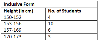
- Inclusive Distribution: When in a distribution, the upper limit does not coincide with the lower limit of the next class then the distribution is called an inclusive distribution. e.g.
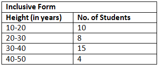
- Exclusive Distribution: An exclusive distribution is that distribution in which the upper limit of one class coincides with the lower limit of the next class. e.g.
- True Class Limit: In the case of exclusive classes the upper and lower limits are respectively known as its true upper limits and true lower limits.
In the case of inclusive classes, the true lower and upper limits are obtained by subtracting 0.5 from the lower limit and adding 0.5 to the upper limit.
True upper limits and true lower limits are also known as boundaries of the class. - Tally: Tally method is used to keep the chance of error at minimum in counting. A bar (|) called tally mark is put against any item when it occurs. The fifth occurrence of any item is represented by putting diagonally a cross tally (|) on the first four tallies.
Frequency Distribution Table
The tabular arrangement of data showing the frequency of each item is called a frequency distribution table. It is a method to present raw data in the form from which one can easily understand the information contained in the raw data.
Frequency distribution are of two types:
- Discrete frequency distribution: In this type of frequency distribution, in the first column of frequency table we write all possible values of the variables from the lowest to the highest, in the second column we write tally marks and in the third column we show frequency of each item. In this method data are not divided into groups or classes.
- Continuous or Grouped Frequency Distribution: In the frequency distribution data are divided into groups or classes. This method is used only where the values in the raw data are largely repeating and the difference between the greatest and the smallest observations is not very large.
Preparation of a frequency distribution table:
The following steps are taken to prepare a frequency distribution table:
- First of all we arrange the data in an array.
- Then draw a table consisting of 3 columns. First column is used for class, the second column for tally and the third column for frequency.
- Then in the first column we write the classes keeping the lowest and the highest scores in view.
- In second column we put tally marks against each class according to the scores.
- Then we write frequency of each class in the third column after counting the tally.
- Figures in first column and third column taken together represent the frequency table.
Cumulative Frequency Table
Cumulative frequency table is obtained from the ordinary frequency table by successively adding the several frequencies. Thus to form a cumulative frequency table we add a column of cumulative frequency in the frequency distribution table. It is obvious that the cumulative frequency of the last class is the sum of the frequencies of all the classes.
Cumulative frequency series are of two types:
- Less than series
- More than series
Graphical Representation of Data
A given data can be represented in graphical way. There are various methods of graphical representation of frequency distribution. Here we shall study only four of them:
- Bar Graphs
- Histogram
- Frequency Polygon
- Cumulative frequency curve or ogive
 |
Download the notes
Statistics and Probability (Part - 1)
|
Download as PDF |
Bar Graphs
The frequency distribution of a discrete value is best represented by a bar graph. The height of the bars is proportional to the frequency of each variate-value. In a bar graph the bars must be kept distinct to show that the variate-values are distinct. The bars are of equal width and are drawn with equal spacing between them on the x-axis depicting the variable. The values of the variable are shown on the y-axis.
Histogram
Histogram is a graphical representation of a grouped frequency distribution with continuous classes. It consists of a set of rectangles where heights of rectangles are proportional to their class frequencies, for equal class intervals. There is no gap between two successive rectangles. The rectangles are constructed with base as the class size and their heights representing the frequencies.
Frequency Polygon
A frequency polygon is a graph of frequency distribution. It is a line graph of class frequency which is plotted against class mark.
A frequency polygon can be obtained by two methods:
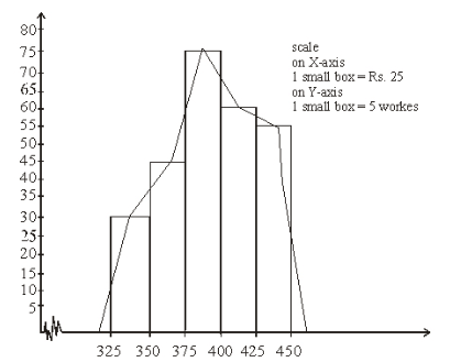
(1) By using Histogram: A frequency polygon can be obtained by joining mid points of the top of the rectangles of a histogram. For this we obtain the mid points of the upper horizontal sides of each rectangle and then join these mid points by dotted lines to get frequency polygon. End of a frequency polygon preferably extended to the mid points of imagined class intervals adjacent to first and last class intervals.
(2) Frequency polygon without using Histogram: Following procedure is used to make a frequency polygon without using histogram.
- Calculate the class marks, x1, x2, ...., xn of each of the given class intervals.
- Mark class marks x1, x2, .... xn, along X-axis and frequencies f1, f2, .... fn along Y-axis.
- Plot the points (x1, f1), (x2, f2), ,....., (xn, fn).
- Obtain the mid-points of two class intervals of zero frequencies at the beginning of the first interval and at the end of the last interval.
- Join the points (x1, f1), (x2, f2), ..., (xn, fn) by the line segments and complete the frequency polygon by joining the mid points of the first and last intervals to the mid points of the imagined classes adjacent to them.
Cumulative frequency curve or ogive
The graphical representation of a cumulative frequency distribution is known as cumulative frequency curve or an ogive.
An ogive can be constructed by following two methods:
Less than method: A less than ogive can be constructed by following steps:
- First of all we make class intervals in exclusive form if it is given in inclusive form.
- Then we construct a less than type cumulative frequency distribution by adding the frequency of each class to the sum of frequencies of its prior classes.
- Now we mark upper class limits along X-axis and cumulative frequencies along Y-axis.(iv) We plot the points (upper class limit, corresponding cumulative frequency) and join them by a free hand curve.
- The lower limit of the first class interval becomes the upper limit of the imagined class with frequency 0. We join the imagined point (lower limit of first class, 0) with the first point of the curve and so on.
In this way we get the required curve called an Ogive by less than type method.
More than Type:
We apply the following steps to construct a more than type ogive:
- Step (1): First of all we make class intervals in exclusive form if it is given in inclusive form.
- Step (2): Then we construct a more than type cumulative frequency distribution.
- Step (3): Now we mark lower lass limits along x-axis and cumulative frequencies along y-axis.
- Step (4): We plot the points (lower class limit, corresponding cumulative frequency) and join them by a free hand curve.
- Step (5): The upper limit of the last class interval becomes the lower limit of the imagined class interval with frequency 0. We join the imagine point (upper limit of last class, 0) with the last point of the curve to end the ogive.
In this way we get the required curve called an ogive by more than type method.
Measures of Central Tendency
An average of a distribution is a single expression which represents a group of variables in a simple and concise manner. It is the representative of entire distribution. Averages are generally in the central parts of the distribution and therefore they are called Measures of Central Tendency.
An ideal measures of central tendency should have following properties:
- It should be defined rigidly.
- It should be based on all observations.
- It should be easy to calculate and readily comprehensible.
- It should be affected as less as possible by fluctuations of sampling.
- Extreme values should not affect very much to measure of central tendency.
Following three types of measures of central tendency are used for analysing data:
- Arithmetic mean
- Median
- Mode
Arithmetic mean for ungrouped data (A. M.)
The arithmetic mean is the most commonly used measure of central tendency. It is obtained by dividing number of observations to the sum of observations. The A. M. of n observations, x1, x2, x3, ......,, xn is given by
A.M = 
Properties of Arithmetic Mean:
- If x is the mean of n observations, x1, x2, ....., xn, then the mean of observations x1 + a, x2 + a, ...., xn + a is , i.e. if each observation is increased by a, then the mean is also increased by a.
- If is the mean of n observations, x1, x2, ..... xn, then the mean of observation, x1 – a, x2 – a, ..., xn – a is i.e. if each observation is decreased by a, then the mean is also decreased by a.
- If is the mean of x1, x2, .... xn then mean of ax1, ax2, .... axn is , where a is any number different from zero i.e. if each observation is multiplied by a non-zero number a, then the mean is also multiplied by a.
- If is the mean of n observations x1, x2, ...., xn then the mean of x1/a, x2/a, ..... xn/a is xÌ„/a where a ≠ 0, i.e. if each observation is divided by a non-zero number, then the mean is also divided by it.
Arithmetic mean of Grouped Data:
Let x1, x2, x3, ..... xn be n observations whose frequencies are f1, f2, f3, .., fn respectively, then the arithmetic mean of this distribution is given by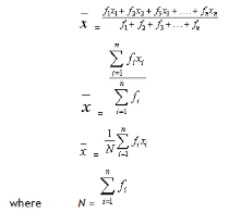
Combined Mean:
Let and be the means of two groups of observations with number of observations n1 and n2 respectively, then the combined mean of two groups is given by,

Merits of Arithmetic Mean:
- A. M. is rigidly defined.
- It is very simple. One can easily understand and calculate it.
- It is uniquely defined.
- It is based upon all the observations.
- A. M. is least affected by sampling fluctuations.
- We can mathematically analysis mean.
- A. M. relatively reliable.
Demerits of Arithmetic Mean:
- A. M. cannot be used for qualitative characteristics like richness, beauty, poverty etc.
- A. M. of a given data can not be determined by inspection. It can be also represented graphically also.
- If any observation is missing then A.M. cannot be calculated.
- A. M. is very much affected by extreme values. In case of extreme items, A. M. gives a distorted picture of the distribution and no longer remains representative of the distribution.
- If the extreme class is open, e.g. below 10 or above 100 then A. M. cannot be calculated.
- If the given data from which the mean has to be calculated, is not given then A. M. may lead to wrong conclusions.
- A. M. cannot be used in the study of ratios, rates etc.
Uses of Arithmetic Mean:
- A. M. is extensively used in practical statistics.
- Estimates can be obtained using A. M.
- A. M. is used for different purposes by different persons like it is used for calculating average marks of the students. It is also used by businessmen to find out profit per unit article, output per machine, average monthly income and expenditure etc.
= 16 – 6
= 10
Hence, f1 = 6 and f2 = 10
Median
Median is defined as the value of that item of the arrayed data which divides the whole data into two equal parts. Hence we have following definition of median:
The middle item of the arrayed data is called its median.
Calculation of median of raw data:
- If the number of observations ‘n’ is odd, then the median will be the value of observation.

- If n is even, then we have two middle terms i.e. (n/2)th observation and (n/2 + 1)th observation.
Median of the given data will be mean of these two middle observations.
|
115 videos|105 docs|110 tests
|
FAQs on Statistics and Probability (Part - 1) - Quantitative for GMAT
| 1. What is the difference between statistics and probability? |  |
| 2. How is probability used in statistics? |  |
| 3. What are the basic concepts in probability theory? |  |
| 4. How is statistics used in decision-making? |  |
| 5. What are the different types of statistical data analysis techniques? |  |


