Solution of Differential Equation | Engineering Mathematics - Engineering Mathematics PDF Download
| Table of contents |
|
| Initial and Boundary value problems |
|
| Laplace Transform |
|
| The Wave equation |
|
| The Diffusion (or heat) Equation |
|

Initial and Boundary value problems
With initial value problems we had a differential equation and we specified the value of the solution and an appropriate number of derivatives at the same point (collectively called initial conditions). For instance for a second order differential equation the initial conditions are,
y(t0) = y0
y'(t0) = y1
With boundary value problems we will have a differential equation and we will specify the function and/or derivatives at different points, which we’ll call boundary values. For second order differential equations, which will be looking at pretty much exclusively here, any of the following can, and will, be used for boundary conditions.
y(x0) = y0 y(x1)= y1
y’(x0) = y0 y’(x1) = y1
y’(x0) = y0 y(x1) = y1
y(x0) = y0 y’(x1) = y1
So, for the purposes of our discussion here we’ll be looking almost exclusively at differential equations in the form,
y'+ p (x) y'+ q(x)y = g(x)
In the earlier chapters, we said that a differential equation was homogeneous if
g(x) = 0
for all x. Here we will say that a boundary value problem is homogeneous if in addition to g(x) = 0 we also have y0 = 0
and y1 = 0 (regardless of the boundary conditions we use). If any of these are not zero we will call the BVP non-homogeneous.
It is important to now remember that when we say homogeneous (or nonhomogeneous) we are saying something not only about the differential equation itself but also about the boundary conditions as well.
When solving linear initial value problems a unique solution will be guaranteed under very mild conditions. With boundary value problems we will often have no solution or infinitely many solutions even for very nice differential equations that would yield a unique solution if we had initial conditions instead of boundary conditions.
So, with some of the basic stuff out of the way let’s find some solutions to a few boundary value problems. Note as well that there really isn’t anything new here yet. We know how to solve the differential equation and we know how to find the constants by applying the conditions. The only difference is that here we’ll be applying boundary conditions instead of initial conditions.
Example 1: Solve the following BVP.
y' + 4y = 0 y(0) = -2 y(π / 4) = 1
Solution:
Okay, this is a simple differential equation so solve and so we’ll leave it to you to verify that the general solution to this is,
y(x) = c1cos(2x) + c2 sin (2x)
Now all that we need to do is apply the boundary conditions.
-2 = y(0) =c1
1 = y (π / 4) =c2
The solution is then,
y(x) = -2cos(2x) + sin(2x)
We mentioned above that some boundary value problems can have no solutions or infinite solutions we had better do a couple of examples of those as well here. This next set of examples will also show just how small of a change to the BVP it takes to move into these other possibilities.
Example 2: Solve the following BVP.
y' + 4y = 0 y(0) = -2 y(2π) = -2
Solution:
We’re working with the same differential equation as the first example so we still have,
y(x) = c1cos(2x) + c2 sin(2x)
Upon applying the boundary conditions we get,
-2 = y(0) = c1
-2 = y(2π) = c1
So in this case, unlike previous example, both boundary conditions tell us that we have to have c1 = 2 and neither one of them tell us anything about
Remember however that all we’re asking for is a solution to the differential equation that satisfies the two given boundary conditions and the following function will do that,
y(x) = -2cos(2x) + c2sin(2x)
In other words, regardless of the value of c2 we get a solution and so, in this case we get infinitely many solutions to the boundary value problem.
Laplace Transform
- Definition and Basic Properties
Initial value problem ⇒ algebra problem ⇒ solution of the algebra problem
⇒ solution of the initial value problem
(i) Definition (Laplace Transform): The Laplace transform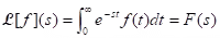 , for all s such that this integral converges.
Examples:

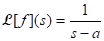 ,
,  .
. 

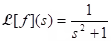 .
.
(ii) Table of Laplace transform of functions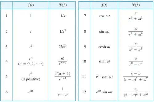 (iii) Theorem (Linearity of the Laplace transform): Suppose
  and
and  are defined for s > a, and ∝ and β are real numbers.
Then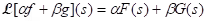 for s > a.
(iv) Definition (Inverse Laplace transform): Given a function G, a function g such that is called an inverse Laplace transform of G. In this event, we write
  .
.
(v) Theorem (Lerch): Let f and g be continuous on [0, ∞) and suppose that . Then f = g.
(vi) Theorem: If and
and  and
and  and
and  are real numbers,
then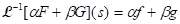
- Solution of initial value problems using the laplace transform
(i) Theorem (Laplace transform of a derivative): Let f be continuous on [0, ∞) and suppose f' is piecewise continuous on [0, k] for every positive k. Suppose also that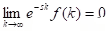 if s > 0. Then
 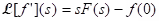 .
.
(ii) Theorem (Laplace transform of a higher derivative): Suppose f, f',...fn - 1 are continuous on [0, ∞) and is piecewise continuous on [0, k] for every positive k. Suppose also that
 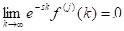 for
for  and for j = 1, 2, ...., n - 1. Then
  .
.
Examples:

 .
.

 .
. - Convolution
(i) Definition (Convolution): If f and g are defined on [0, ∞), then the convolution f * g of f with g is the function defined by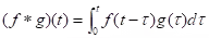 for t ≥ 0.
(ii) Theorem (Convolution theorem): If f * g is defined, then .
.
(iii) Theorem: Let and
and  . Then
  .
.
Example:

 .
.
Determine f such that

 .
.
(iv) Theorem: If is defined, so is
  , and
, and  .
.
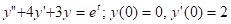
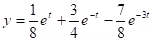
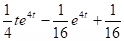
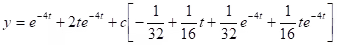
Example: Solve

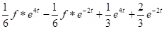 .
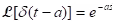
. - Unit impulses and the dirac’s delta function
(i) Dirac’s delta function: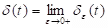 where;
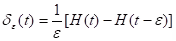
 ;
;  .
.
(ii) Theorem (Filtering property): Let a > 0 and let f be integrable on [0, ∞) and continuous at a. Then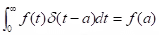
Let the

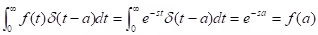
 definition of the Laplace transformation of the delta function.
Example: Solve

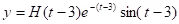 .
.
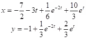
(iii) Laplace Transform Solution of Systems:
Example: Solve the system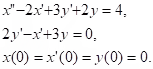

(iv) Differential Equations with Polynomial Coefficients
(a) Theorem: Let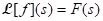 for s > b and suppose that F is differentiable. Then
 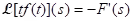 for s > b.
(b) Corollary: Let for s > b and let n be a positive integer. Suppose F is n times differentiable. Then
 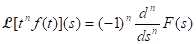 for s > b.
Example:

 .
.
(c) Theorem: Let f be piecewise continuous on for every positive number k and suppose there are numbers M and b such that
  for t ≥ 0. Let
 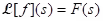 . Then
  .
.
Example:

 .
.
The Wave equation
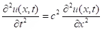 - one dimensional wave equation.
The variable t has the significance of time, the variable x is the spatial variable. Unknown function u(x,t) depends both of x and t. For example, in case of vibrating string the function u(x,t) means the string deviation from equilibrium in the point x at the moment t.
Consider the wave equation for the vibrating string in more details.
Applying the 2d Newton’s law to the portion of the string between points x and x → Δx we get the equation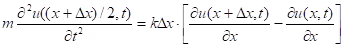
and dividing by the Δx and taking the limit Δx → o we obtain the wave equation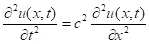 (1)
(1)
If both ends of the string are fixed then the boundary conditions are
u(0, t) = 0, u(1, t) = 0
and the initial conditions are In case of infinite string - ∞ < x < ∞, t > 0 the wave equation with initial conditions has solution (D’Alembert’s solution):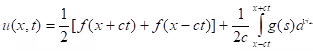
The Diffusion (or heat) Equation
The equation for this distribution is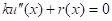
Now we consider the temperature distribution  , which depends on the point x of the rod and time t.
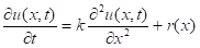
In case of diffusion equation r(x)=0.
Initial temperature distribution u(x, 0) = f(x).
If the function f(x) is so-called delta function (at initial moment we have the heat source at one point with coordinate ξ) then the homogeneous (r(x) = 0) heat equation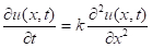
has the solution. 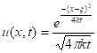
This is the so-called fundamental solution.
Example: The Braselton (chemical reaction system with two components) on the unit interval.
Solution: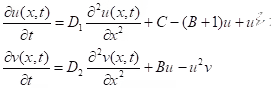
x ∈ [0,1]; D1, D2, B, C > 0
u(0, t) = u(1, t) = C, v(0, t) = v(1, t) = B / C
|
65 videos|129 docs|94 tests
|


shortcuts and tricks
,Solution of Differential Equation | Engineering Mathematics - Engineering Mathematics
,Semester Notes
,past year papers
,Free
,Previous Year Questions with Solutions
,Solution of Differential Equation | Engineering Mathematics - Engineering Mathematics
,Sample Paper
,Extra Questions
,mock tests for examination
,practice quizzes
,study material
,video lectures
,ppt
,MCQs
,Solution of Differential Equation | Engineering Mathematics - Engineering Mathematics
,Exam
,Viva Questions
,Summary
,Important questions
,Objective type Questions
;


Solution of Differential Equation Free PDF Download
Importance of Solution of Differential Equation
Solution of Differential Equation Notes
Solution of Differential Equation Engineering Mathematics Questions
Study Solution of Differential Equation on the App
|
© EduRev
|
Education Revolution
|


|


