Time Domain Analysis of First Order and Second Order System | Control Systems - Electrical Engineering (EE) PDF Download
Time Domain Analysis
The Time Domain Analyzes of the system is to be done on basis of time. The analysis is only be applied when nature of input plus mathematical model of the control system is known. Expressing the main input signals is not an easy task and cannot be determined by simple equations. There are two components of any system’s time response, which are: Transient response & Steady state response.
- Transient Response: This response is dependent upon the system poles only and not on the type of input & it is sufficient to analyze the transient response using a step input.
- Steady-State Response: This response depends on system dynamics and the input quantity. It is then examined using different test signals by final value theorem.


Standard Test Input Signals
1. Step Input Signal:

Let us take an independent voltage source or a battery which is connected across a voltmeter via a switch, s. It is clear from the figure below, whenever the switch s is open, the voltage appears between the voltmeter terminals is zero. If the voltage between the voltmeter terminals is represented as v (t), the situation can be mathematically represented as Now let us consider at t = 0, the switch is closed and instantly the battery voltage V volt appears across the voltmeter and that situation can be represented as,
Combining the above two equations we get In the above equations if we put 1 in place of V, we will get a unit step function which can be defined as
 Let’s examine the Laplace transform of the unit step function. To find the Laplace transform of any function, multiply it by e-st and integrate from 0 to infinity.
 If input is R(s), then
2. Ramp Function:
A ramp function is represented by a straight line starting from the origin and inclining upwards. It begins at zero and increases or decreases linearly over time. Here in this above equation, k is the slope of the line.
 Unit Ramp SignalNow let us examine the Laplace transform of ramp function. As we told earlier Laplace transform of any function can be obtained by multiplying this function by e-st and integrating multiplied from 0 to infinity.

3. Parabolic Function:
Here, the value of function is zero when time t<0 and is quadratic when time t > 0. A parabolic function can be defined as, Now let us examine the Laplace transform of parabolic function. As we told earlier Laplace transform of any function can be obtained by multiplying this function by e-st and integrating multiplied from 0 to infinity.

 Unit Parabolic Signal

Time-Response of First-Order System
Here consider the armature-controlled dc motor driving a load, such as a video tape. The objective is to drive the tape at a constant speed. Note that it is an open-loop system. 


- ωss(t) is the steady-state final speed. If the desired speed is ωr, choosing 'a=ωr/k1km' the motor will eventually reach the desired speed.
- From the time response e-t/τm we concluded that for t≥5τm the value of e-t/τm is less than 1% of its original value. Hence the speed of the motor will reach and stay within 1% of its final speed at 5 time constants.

Let us now consider the closed-loop system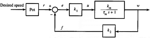


If r(t) = a then Response would be ; w(t) = ak1ko - ak1koe - t / τo
If a is properly chosen, the tape can reach a desired speed. It will reach the desired speed in 5τo seconds. Here τo=τm. So that we can control the speed of response in the feedback system.
Ramp response of first-order system
Let, k1k0 = 1 for simplicity. Then, T(s) = (1/(τ0s + 1)) = W(s) / R(s). Also, let r(t) = tu(t)
Then, W(s)= 
⇒ w(t) = tu(t) - τ0(1 - e-t/τ0)u(t)
The error signal is, e(t) = r(t) - w(t)
Or, e(t) = τ0(1 - e-t/τ0)u(t)
ess(t) = τo
- Thus, the first-order system will track the unit ramp input with a steady-state error τo, which is equal to the time-constant of the system.
Time-Response of Second-Order System
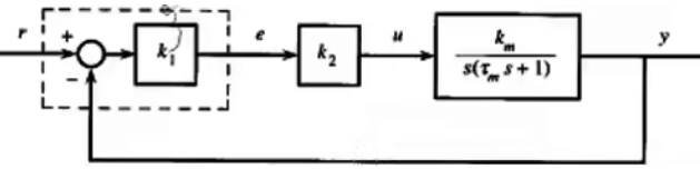
- Consider the antenna position control system. Its transfer function from r to y is,
where we can define
(ωn)2 = k1k2km / τm ; & 2ξωn = 1 / τm
The constant ξ is called the damping ratio and ωn is called the natural frequency. The system above is, in fact, a standard second order system.
The transfer function T(s) has two poles and no zero. Its poles are,


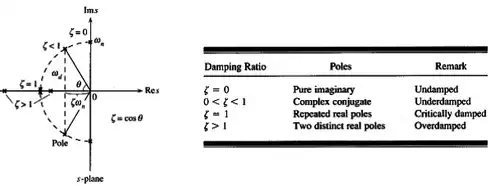
Natural frequency (ωn): The natural frequency of a second order system is the frequency of oscillation of the system without damping.
Damping ratio (ξ): The damping ratio is defined as the ratio of the damping factor σ, to the natural frequency ωn.
Here,σ is called the damping factor,ωd is called damped or actual frequency. The location of poles for different ξ are plotted in the given figure below. For ξ=0, the two poles ±jωn are purely imaginary. If 0<ξ<1, the two poles are complex conjugate.
Unit Step Response of Second-Order System
Suppose, r(t) = u(t), ⇒ R(s) = 1/s; 
Or
Performing inverse Laplace transform,


Second-Order Systems: General Specification
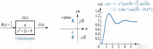
Second order system exhibits a wide range of responses that must be analyzed and described. To become familiar with the wide range of responses before formalizing our discussion, we take a look at numerical examples of the second order system responses shown in the figure.
- Underdamped Response (0 < ξ < 1)
This function has a pole at the origin that comes from the unit step and two complex poles that come from the system. The sinusoidal frequency is given the name of damped frequency of oscillation, ωd. This response shown in figure called underdamped.
Example: - Overdamped System (1 < ξ)
This function has a pole at the origin that comes from the unit step input and two real poles that come from the system. The input pole at the origin generates the constant forced response; each of two system poles on the real axis generates an exponential natural frequency.
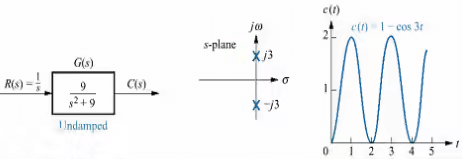
Example: - Undamped Response (ξ = 0)
This function has a pole at the origin and two imaginary poles. The pole at the origin generates the constant forced response, and the two system poles on the imaginary axis at ±j3 generate a Sinusoidal natural response.
Example: - Critically Damped Response (ξ = 1)
This function has a pole at the origin and two multiple real poles. The input pole at the origin generates the constant forced response, and two poles at the real axis at -3 generate a natural exponential response.


Note: In the above specifications of time domain, don't be confused with the number of Poles in G(s), to Specify for which type of Damping is present for a particular case we consider the total number of poles are of transfer function i.e; C(s) / R(s).
Summarization: Here once again we summarize the second order damping functions as;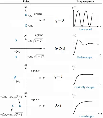
Time Domain Characteristics
In specifying the Transient-Response characteristics of a control system to a unit step input, we usually specify the following:- Delay time (td): It is the time required for the response to reach 50% of the final value in first attempt.
- Rise time, (tr): It is the time required for the response to rise from 0 to 100% of the final value for the underdamped system.
- Peak time, (tp): It is the time required for the response to reach the peak of time response or the peak overshoot.
- Settling time, (ts): It is the time required for the response to reach and stay within a specified tolerance band ( 2% or 5%) of its final value.
- Peak overshoot (Mp): It is the normalized difference between the time response peak and the steady output and is defined as
- Steady-state error (ess): It indicates the error between the actual output and desired output as ‘t’ tends to infinity.
- Rise time, t,: Put y(t) = 1 at t = tr, ⇒ sin(ωdtr + θ) = 0 = sinπ, ⇒ tr = (π - θ) / ωd ; θ = cos-1ξ
- Peak time, tp : Put dy / dt = 0 and solve for t = tp : 0 = (σωn / ωd)e-at sin(ωdt + θ) - ωne-at cos(ωdt + θ)
Peak overshoot occurs at k = 1. ⇒ tp = π/ωd = π/ωn.
Settling time, ts : For 2% tolerance band,


 .
.
Steady-state error ess: It is found previously that steady-state error for step input is zero. Let us now consider ramp input, r(t) = tu(t).
- Therefore, the steady-state error due to ramp input is 2ξ / ωn.
Effect of Adding a Zero to a System
If we add a zero at s = -z be added to a second order system. Then we have,
- The multiplication term is adjusted to make the steady-state gain of the system unity.
Manipulation of the above equation gives, - The effect of added derivative term is to produce a pronounced early peak to the system response.
- Closer the zero to the origin, the more pronounce the peaking phenomenon.
- Due to this fact, the zeros on the real axis near the origin are generally avoided in design. However, in a sluggish system the artful introduction of a zero at the proper position can improve the transient response.


Types of Feedback Control System
The open-loop transfer function of a system can be written as
- If n = 0, the system is called type-0 system, if n = 1, the system is called type-1 system, if n = 2, the system is called type-2 system, etc.
Steady-State Error and Error Constants
The steady-state performance of a stable control system is generally judged by its steady-state error to step, ramp and parabolic inputs. For a unity feedback system,
It is seen that steady-state error depends upon the input R(s) and the forward transfer function G(s).
- For unit-step input: r(t) = u(t), R(s) = 1 / s kP is called position error constant.
- For unit-ramp input : r(t) = tu(t), R(s) = 1 / s2kv is called velocity error constant.
- For unit-parabolic input: r(t) = t2 / 2, R(s) = 1 / s3 is called acceleration error const.
 kP is called position error constant.
 kv is called velocity error constant.
 is called acceleration error const.
|
53 videos|73 docs|40 tests
|
FAQs on Time Domain Analysis of First Order and Second Order System - Control Systems - Electrical Engineering (EE)
| 1. What is time domain analysis? |  |
| 2. What is the time-response of a first-order system? | |
| 3. How is the time-response of a second-order system different from a first-order system? | |
| 4. What is the unit step response of a second-order system? | |
| 5. What are the time domain characteristics analyzed in a first-order system? | |

|
4.83/5 Rating |

|
Dec 29, 2024 Last updated |

|
Explore Courses for Electrical Engineering (EE) exam
|
|
practice quizzes
,Semester Notes
,Objective type Questions
,past year papers
,Exam
,Summary
,Time Domain Analysis of First Order and Second Order System | Control Systems - Electrical Engineering (EE)
,video lectures
,Previous Year Questions with Solutions
,ppt
,Time Domain Analysis of First Order and Second Order System | Control Systems - Electrical Engineering (EE)
,Sample Paper
,Time Domain Analysis of First Order and Second Order System | Control Systems - Electrical Engineering (EE)
,MCQs
,study material
,Important questions
,Free
,mock tests for examination
,shortcuts and tricks
,Viva Questions
,Extra Questions
;


Time Domain Analysis of First Order and Second Order System Free PDF Download
Importance of Time Domain Analysis of First Order and Second Order System
Time Domain Analysis of First Order and Second Order System Notes
Time Domain Analysis of First Order and Second Order System Electrical Engineering (EE) Questions
Study Time Domain Analysis of First Order and Second Order System on the App
|
© EduRev
|
Education Revolution
|


|


