Polar Plots | GATE Notes & Videos for Electrical Engineering - Electrical Engineering (EE) PDF Download
Polar plot is a plot which can be drawn between magnitude and phase. Here, the magnitudes are represented by normal values only.
The polar form of G(jω)H(jω) is:
G(jω)H(jω) = |G(jω)H(jω)|∠G(jω)H(jω)
Definition: The polar plot of a sinusoidal transfer function is the plot of the magnitude G(jω) versus the phase angle of G(jω) on the polar coordinates. The frequency(ω) in the polar plot is varied from zero to infinity.
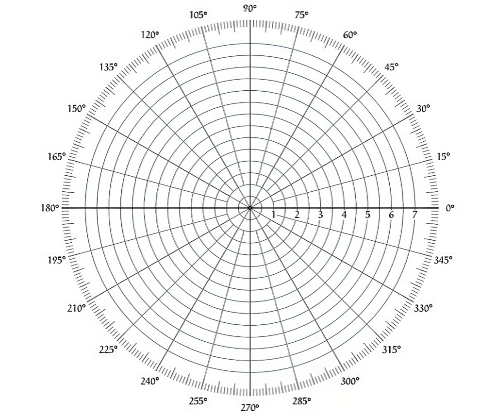 Polar Graph Sheet
- The polar plot is drawn on the polar sheet, which is the form of a graph, and the graph consists of concentric circles and radial lines.
- The concentric circles on the polar sheet graph represent the magnitude, and the radial lines represent phase angles. Each point on the graph displays information about the magnitude and the phase angle.
The example of a polar graph is shown below:
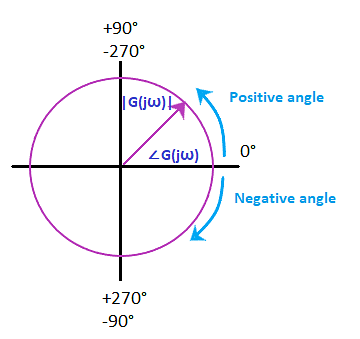
- The positive angle in a polar graph is measured in the anti-clockwise direction, while the negative angle is measured clockwise direction. Both the angles are measured with respect to the reference point, i.e., 0 degree axis.
The transfer function G(jω) in the rectangular form can be written as:
G(jω) = GR(jω) + GI(jω)
Where,
- GR(jω) is the real part of the transfer function G(jω)
- GI(jω) is the imaginary part of the transfer function G(jω)
Note: As discussed, the angular frequency in the polar plot varies from zero to infinity. We should not get confused with the Nyquist plot, which is the extension of the polar plot. The angular frequency (ω) varies from zero to infinity, while the Nyquist plot varies from a negative value of infinity to positive infinity.
The primary advantage of the polar plot is that it depicts the frequency response characteristics of a system over the entire frequency range in a single plot. Since everything seems to be a single block, it fails to show the contributions of each factor of the open-loop transfer function.
The integral factor of the polar plot is given by:
G(s) = 1/s
Where,
s = jω; s is the transfer function
G(jω) = 1/jω (It is the negative imaginary axis.)
The derivative factor of the polar plot is given by:
G(jω) = jω (It is the positive imaginary axis.)
Effect of Addition of Pole and Zero
- The addition of pole in the polar plot will shift its end by -90 degrees.
- The addition of zero in the polar plot will shift its end by +90 degrees.
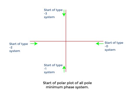
Type and Order of the System
The type of the system in the polar plot determines the quadrant at which the polar plot starts. The start of the polar plot of all poles is shown in the below diagram.
Order of the System: The order of the system in the polar plot determines the quadrant at which the polar plot ends. The end of the polar plot of all poles is shown in the below diagram.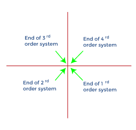
Procedure to Sketch the Polar Plot
- Step-1: Determine transfer function G(jω).
- Step-2: Put s = jω in the transfer function to obtain G(jω).
- Step-3: At ω = 0 and m = ∞, calculate |G(jω)| by
 and . .
 - Step-4: Calculate the phase angle of G(jω) at ω = 0 and ω = ∞ and .
- Step-5: Rationalize the function G(jω) and separate the real and imaginary axis.
- Step-6: Equate the imaginary part Im|G(jω)| to zero and determine the frequencies at which plot intersects the real axis and calculate the value of G(jω) at the point of intersection by substituting the determined value of frequency in the expression of G(jω).
- Step-7: Equate the real part Re|G(jω)| to zero and determine the frequencies at which plots intersects the imaginary axis and calculate the value G(jω) at the point of intersection by substituting the determined value of frequency in the rationalized expression of G(jω).
- Step-8: Sketch the polar plot with the help of above information.
 and
and 

 .
.Polar Plot of Some Standard Transfer Functions:
(a) Type 0
Order 1
Let, G(s) = 1/(1 + sT)
Put, s= jω
G(jω) = 1/(1 + jωT)
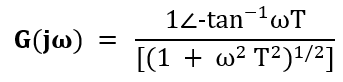
- The above transfer function in the form of magnitude and angle can be represented as:
- If we consider the angle part in the numerator, we need to insert a negative sign due to the transition from the denominator to the numerator or vice-versa.
Let's find the value of the above function at zero and infinity.
- When, ω = 0
G(jω) = 1∠0/1
G(jω) = 1∠0
It is because tan-10 = 0 - When, ω = infinity
G(jω) = 0∠-90
It is because tan-1 ∞ = 90 degrees
The polar plot at value 0 and infinity will appear as:

Order 2
Since, it is a 2 order system; the function includes the highest derivative variable (s) with the power 2.
Let,
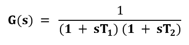
Put, s= jω
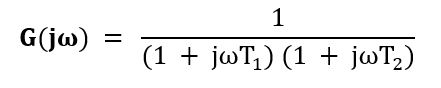
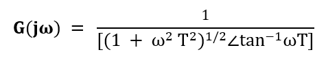
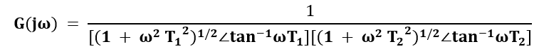
- The above transfer function in the form of magnitude and angle can be represented as:
- If we consider the angle part in the numerator, we need to insert a negative sign due to the transition from the denominator to the numerator, as shown below:
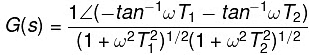
G(jω) = 1∠(-tan-1ωT1 - tan-1ωT2) /(1 + ω2 T1 2)1/2(1 + ω2 T2 2)1/2
Let's find the value of the above function at zero and infinity.
- When, ω = 0
G(jω) = 1∠(-0 - 0)/1x1
G(jω) = 1∠0
It is because tan-10 = 0 - When, ω = infinity
G(jω) = 0∠(-90 - 90)/1
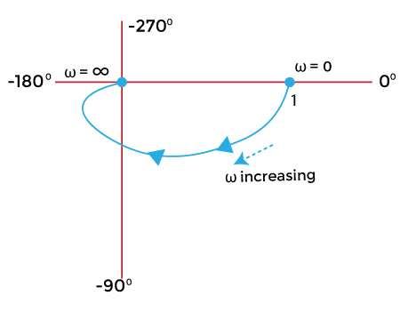
G(jω) = 0∠-180
It is because tan-1 ∞ = 90 degrees
The polar plot at value 0 and infinity will appear as:
(b) Type 1
 (b) Type 1
Order 1
Let, G(s) = 1/s
Put, s= jω
G(jω) = 1/jω
G(jω) = 1/(ω∠90)
- If we consider the angle part in the numerator, we need to insert a negative sign due to the transition from the denominator to the numerator, as shown below:
G(jω) =1∠-90 /ω
Let's find the value of the above function at zero and infinity.
- When, ω = 0
G(jω) =∞ ∠-90
It is because the function is directly divided by ω. 1/0 = infinity.
tan-10 = 0 - When, ω = infinity
G(jω) = 0∠-90
It is because the function is directly divided by ω. 1/infinity = zero.
tan-1 ∞ = 90 degrees
The polar plot at value 0 and infinity will appear as:
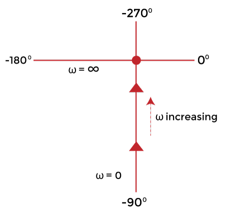
Order 2
Let, G(s) = 1/s(1 + sT)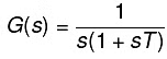
Put, s= jω
G(jω) = 1/ jω(1 + jωT)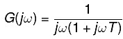
- The above transfer function in the form of magnitude and angle can be represented as:
G(jω) = 1/ω∠90 [(1 + ω2 T2)1/2∠tan-1ωT] - If we consider the angle part in the numerator, we need to insert a negative sign due to the transition from the denominator to the numerator or vice-versa.
G(jω) = 1∠(-90 - tan-1ωT) / ω(1 + ω2 T2)1/2
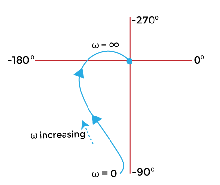
Let's find the value of the above function at zero and infinity.
- When, ω = 0
G(jω) =∞ ∠-90
It is because the function is directly divided by ω. 1/0 = infinity.
tan-10 = 0 - When, ω = infinity
G(jω) = 0∠(-90-90)
G(jω) = 0∠-180
It is because the function is directly divided by ω. 1/infinity = zero.
tan-1 ∞ = 90 degrees
The polar plot at value 0 and infinity will appear as:
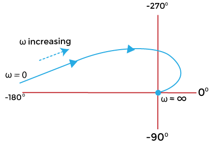
Order 3
Let, G(s) = 1/s(1 + sT1) (1 + sT2)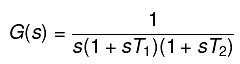
Put, s= jω
G(jω) = 1/ jω (1 + jωT1) (1 + jωT2)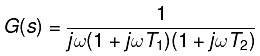
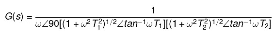
- The above transfer function in the form of magnitude and angle can be represented as:
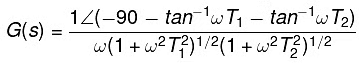
G(jω) = 1/ ω∠90 [(1 + ω2 T1 2)1/2∠tan-1ωT1][( 1 + ω2 T2 2)1/2∠tan-1ωT2] - If we consider the angle part in the numerator, we need to insert a negative sign due to the transition from the denominator to the numerator, as shown below:
G(jω) = 1∠(-90 -tan-1ωT1 - tan-1ωT2) /ω(1 + ω2 T12)1/2(1 + ω2 T22)1/2
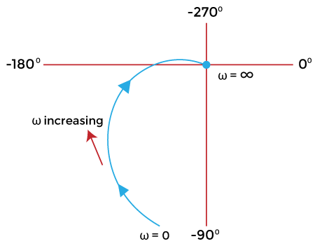
Let's find the value of the above function at zero and infinity.
- When, ω = 0
G(jω) =∞ ∠-90
It is because the function is directly divided by ω. 1/0 = infinity.
tan-10 = 0 - When, ω = infinity
G(jω) = 0∠(-90 -90 -90)
G(jω) = 0∠-270
It is because the function is directly divided by ω. 1/infinity = zero.
tan-1 ∞ = 90 degrees
The polar plot at value 0 and infinity will appear as:
(c) Type 2
Order 4
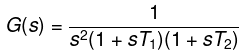
Put, s= jω
G(jω) = 1/ j2 ω2 (1 + jωT1) (1 + jωT2)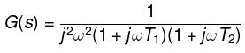
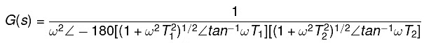
- The above transfer function in the form of magnitude and angle can be represented as:
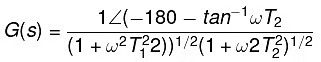
G(jω) = 1/ ω2∠-180 [(1 + ω2 T1 2)1/2∠tan-1ωT1][( 1 + ω2 T2 2)1/2∠tan-1ωT2] - If we consider the angle part in the numerator, we need to insert a negative sign due to the transition from the denominator to the numerator, as shown below:
G(jω) = 1∠(-180-tan-1ωT1 - tan-1ωT2) /(1 + ω2 T1 2)1/2(1 + ω2 T22)1/2
Let's find the value of the above function at zero and infinity.
- When, ω = 0
G(jω) = ∞ ∠(-180 - 0 - 0)/1x1
G(jω) = ∞ ∠-180
It is because the function is directly divided by ω. 1/0 is equal to infinity.
tan-10 = 0 - When, ω = infinity
G(jω) = 0∠(-180 - 90 - 90)/1
G(jω) = 0∠-360
It is because the function is directly divided by ω. 1/infinity is equal to zero.
tan-1 ∞ = 90 degrees
The polar plot at value 0 and infinity will appear as:
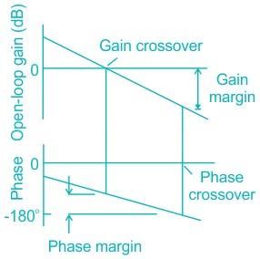
Gain Margin and Phase Margin of Polar Plot
- Phase Crossover Frequency: The frequency at which the polar plot crosses the -180° line is called phase crossover frequency.
- Gain Crossover Frequency: The frequency at which the polar plot crosses the unity circle is called gain crossover frequency.
- Gain Margin: At phase crossover frequency, if gain is 'a' then
Gain margin = - 20 log a - Phase Margin (φm): At gain crossover frequency, if phase is φ then phase margin φm = 180 + φ
where, φ is positive from anti-clockwise direction.

The gain margin is Kg. It is given by:
Kg = 1/GB
- GB is the value at a point (B) on the magnitude circle that cuts the 180 degree axis.
- The gain margin is positive if the point B lies within unit circle. Otherwise, it is negative.
The phase margin is given by:
Y = 180 + theta
Where,
- Theta is the phase angle of G(jω) at the gain crossover frequency. The phase angle is calculated when the magnitude curve line intersects with the external unity circle. The line drawn from that intersection point to the end of the graph determines the angle theta. It can be positive or negative.
Both the phase margin and the gain margin can be better understood with the help of an example.
Let's discuss an example of the polar plot.
Example: The open loop transfer function of a unity feedback system is given by G(s) = 1/s(s + 1)(2s + 1). Sketch the polar plot and also determine the gain margin and the phase margin.
The transfer function is given by:
G(s) = 1/s(s + 1)(2s + 1)
The above function clearly depicts that the system is of type 1 and order 3. It is in the form:
G(s) = 1/s(1 + sT1) (1 + sT2)
Put, s = jω
G(s) = 1/ jω (jω + 1)(2jω + 1)
The above transfer function in the form of magnitude and angle can be represented as:
G(jω) = 1/ ω∠90 [(1 + ω2)1/2∠tan-1ω][( 1 + ω24)1/2∠tan-1ω2]
If we consider the angle part in the numerator, we need to insert a negative sign due to the transition from the denominator to the numerator, as shown below:
Now, let us separate the magnitude and angle terms from the above equation.
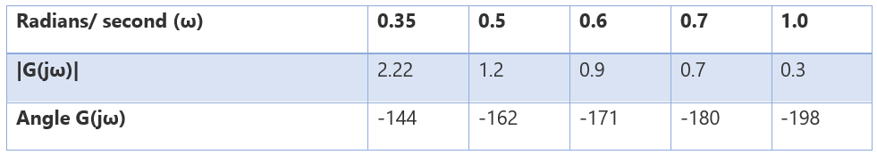
|G(jω)| = 1/ ω((1 + ω2) (1 + 4ω2))1/2
|G(jω)| = 1/ ω(1 + 4ω2 + ω2+ 4ω4)1/2
|G(jω)| = 1/ ω(1 + 5ω2 + 4ω4)1/2
Angle G(jω) = -90 -tan-1ω - tan-1 2ω
We know the value of the above function at zero and infinity.
When, ω = 0
G(jω) =∞ ∠-90
When, ω = infinity
G(jω) = 0∠-270
Let's find the magnitude and phase of G(jω) at different frequencies.
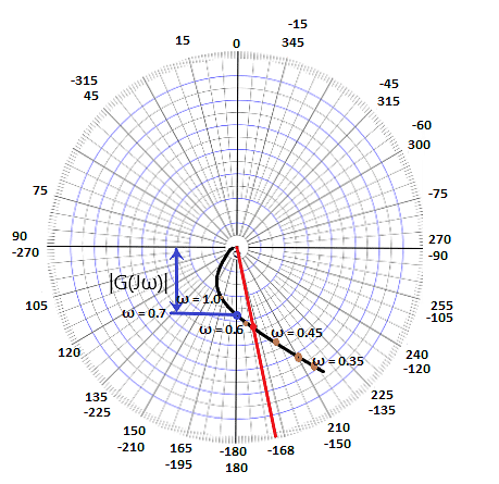
The polar plot is shown below:
Here, every two lines have a gap of 15 degrees. We have specified both the positive and negative angle value at a point. It is based on the concept that the positive angles are measured anti-clockwise and the negative angles are measured clockwise. As we start from the 0 angle in the clockwise direction, we can notice the increase in the negative values of the angle. Similarly, as we begin from the 0 angle in the clockwise direction, we can notice the rise in the positive values of the angle.
Let's calculate the gain margin and the phase margin.
We can see in the polar plot that the magnitude circle cuts the 180 degree axis at point 0.7. Hence, it will be the value of GB.
The gain margin is Kg = 1/GB
Kg = 1/0.7
Kg = 1.428
The phase margin is given by:
Y = 180 + theta
We can clearly see the point marked with the red color. It is the intersection point of the magnitude curve with the unity circle. The line drawn from the intersection point (marked in red) determines the theta angle, which is equal to (-168) degrees.
So, phase angle is equal to
Y = 180 - 168
Y = 12 degrees
Thus, the gain margin is 1.428 and the phase angle is 12 degrees.


|
27 videos|328 docs
|
FAQs on Polar Plots - GATE Notes & Videos for Electrical Engineering - Electrical Engineering (EE)
| 1. What is a polar plot in electrical engineering? |  |
| 2. How is the gain margin related to the polar plot? | |
| 3. What is the phase margin in a polar plot? | |
| 4. How can the polar plot be sketched? | |
| 5. What information can be obtained from a polar plot? | |

|
4.65/5 Rating |

|
Dec 22, 2024 Last updated |
|
27 videos|328 docs
|

|
Explore Courses for Electrical Engineering (EE) exam
|
|
Polar Plots | GATE Notes & Videos for Electrical Engineering - Electrical Engineering (EE)
,Semester Notes
,past year papers
,Sample Paper
,mock tests for examination
,video lectures
,Viva Questions
,ppt
,Summary
,Free
,Objective type Questions
,Exam
,Extra Questions
,Polar Plots | GATE Notes & Videos for Electrical Engineering - Electrical Engineering (EE)
,shortcuts and tricks
,MCQs
,Polar Plots | GATE Notes & Videos for Electrical Engineering - Electrical Engineering (EE)
,Important questions
,Previous Year Questions with Solutions
,study material
,practice quizzes
;


Polar Plots Free PDF Download
Importance of Polar Plots
Polar Plots Notes
Polar Plots Electrical Engineering (EE) Questions
Study Polar Plots on the App
|
© EduRev
|
Education Revolution
|


|


