Class 6 Exam  >  Class 6 Notes  >  How to become an Expert of MS Excel  >  How to Use Excel's VLOOKUP Function

How to Use Excel's VLOOKUP Function | How to become an Expert of MS Excel - Class 6 PDF Download

Introduction

Many of our learners have told us they want to learn how to use Excel's VLOOKUP function. VLOOKUP is an extremely useful tool, and learning how to use it is easier than you think!

What exactly is VLOOKUP?

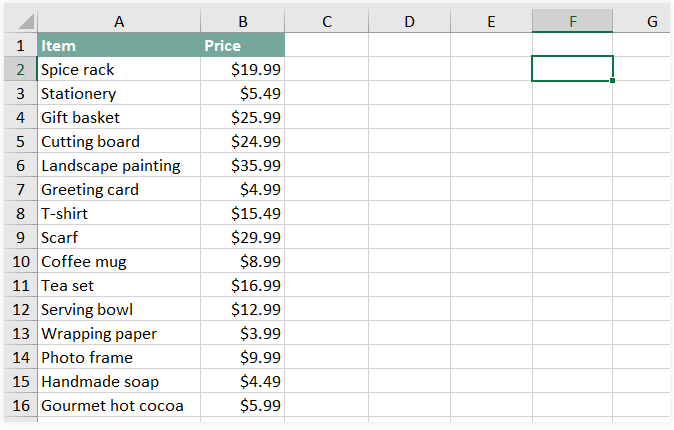
  • Basically, VLOOKUP lets you search for specific information in your spreadsheet. For example, if you have a list of products with prices, you could search for the price of a specific item.
  • We're going to use VLOOKUP to find the price of the Photo frame. You can probably already see that the price is $9.99, but that's because this is a simple example. Once you learn how to use VLOOKUP, you'll be able to use it with larger, more complex spreadsheets, and that's when it will become truly useful.
    How to Use Excel`s VLOOKUP Function | How to become an Expert of MS Excel - Class 6
  • We'll add our formula to cell F2, but you can add it to any blank cell. As with any formula, you'll start with an equals sign (=). Then type the formula name. Our arguments will need to be in parentheses, so type an open parenthesis. So far, it should look like this:
    = VLOOKUP(

Adding the arguments

Now, we'll add our arguments. The arguments will tell VLOOKUP what to search for and where to search.

  • The first argument is the name of the item you're searching for, which in this case is Photo frame. Because the argument is text, we'll need to put it in double quotes:
    =VLOOKUP("Photo frame"
  • The second argument is the cell range that contains the data. In this example, our data is in A2:B16. As with any function, you'll need to use a comma to separate each argument:
    =VLOOKUP("Photo frame", A2:B16

It's important to know that VLOOKUP will always search the first column in this range. In this example, it will search column A for "Photo frame". The value that it returns (in this case, the price) will always need to be to the right of that column.

  • The third argument is the column index number. It's simpler than it sounds: The first column in the range is 1, the second column is 2, etc. In this case, we are trying to find the price of the item, and the prices are contained in the second column. This means our third argument will be 2:
    =VLOOKUP("Photo frame", A2:B16, 2
  • The fourth argument tells VLOOKUP whether to look for approximate matches, and it can be either TRUE or FALSE. If it is TRUE, it will look for approximate matches. Generally, this is only useful if the first column has numerical values that have been sorted. Because we're only looking for exact matches, the fourth argument should be FALSE. This is our last argument, so go ahead and close the parentheses:
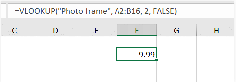
    =VLOOKUP("Photo frame", A2:B16, 2, FALSE)

That's it! When you press Enter, it should give you the answer, which is 9.99.
How to Use Excel`s VLOOKUP Function | How to become an Expert of MS Excel - Class 6

How it works

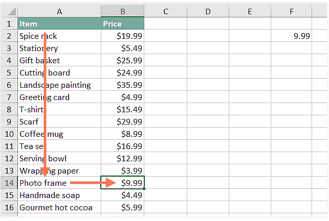
Let's take a look at how this formula works. It first searches vertically down the first column (VLOOKUP is short for vertical lookup). When it finds "Photo frame", it moves to the second column to find the price.

How to Use Excel`s VLOOKUP Function | How to become an Expert of MS Excel - Class 6

As we mentioned earlier, the price needs to be to the right of the item name. VLOOKUP cannot look to the left of the column that it's searching.
If we want to find the price of a different item, we can just change the first argument:
=VLOOKUP("T-shirt", A2:B16, 2, FALSE)
or:
=VLOOKUP("Gift basket", A2:B16, 2, FALSE)
It would be very tedious to edit your VLOOKUP formula whenever you want to find the price of a different item. In the next example, we'll show how to avoid this by using a cell reference.

Another example

Are you ready for a slightly more advanced example? We're going to make a couple of changes to the spreadsheet to make it more realistic.

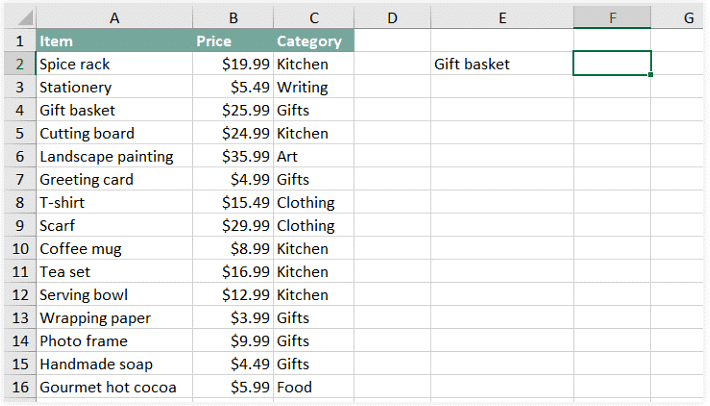
  • In the previous example, we typed the item name directly into the VLOOKUP formula. But in the real world, you'll usually use a cell reference instead. In this example, we'll type the item name in cell E2, and our VLOOKUP formula can then use a cell reference to find information about that product. Then, we can simply type a new item name into E2 to find any product we want.
  • We've also added a third column that has the category for each item. This will give us the option of finding the price or category. Here's what the spreadsheet looks like so far:
    How to Use Excel`s VLOOKUP Function | How to become an Expert of MS Excel - Class 6
  • Our formula will be similar to the previous example, but we'll need to change the first three arguments. Let's start by changing the first argument to a cell reference (make sure to remove the quotation marks):
    =VLOOKUP(E2, A2:B16, 2, FALSE)
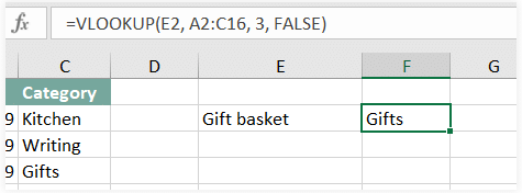
  • To find the category, we'll need to change the second and third arguments. First, we'll change the range to A2:C16 so it includes the third column. Next, we'll change the column index number to 3 because our categories are in the third column:
    =VLOOKUP(E2, A2:C16, 3, FALSE)
  • When you press Enter, you'll see that the Gift basket is in the Gifts category.
    How to Use Excel`s VLOOKUP Function | How to become an Expert of MS Excel - Class 6
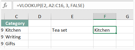
  • If we want to find the category of a different item, we can simply change the item name in cell E2:
    How to Use Excel`s VLOOKUP Function | How to become an Expert of MS Excel - Class 6
The document How to Use Excel's VLOOKUP Function | How to become an Expert of MS Excel - Class 6 is a part of the Class 6 Course How to become an Expert of MS Excel.
All you need of Class 6 at this link: Class 6
94 videos|62 docs|15 tests

Top Courses for Class 6

FAQs on How to Use Excel's VLOOKUP Function - How to become an Expert of MS Excel - Class 6

1. What is the VLOOKUP function in Excel?
Ans. The VLOOKUP function in Excel is a powerful tool that allows users to search for a specific value in a range of cells and return a corresponding value from another column. It is commonly used to retrieve data from large datasets or lookup tables.
2. How do I use the VLOOKUP function in Excel?
Ans. To use the VLOOKUP function in Excel, follow these steps: 1. Select the cell where you want the result to be displayed. 2. Type "=VLOOKUP(" in the formula bar. 3. Specify the value you want to lookup. 4. Specify the range of cells where the lookup should be performed. 5. Specify the column index number of the value you want to retrieve. 6. Specify whether you want an exact match or an approximate match. 7. Close the formula with a closing parenthesis. 8. Press Enter to get the result.
3. Can the VLOOKUP function search for values in multiple columns?
Ans. No, the VLOOKUP function can only search for values in a single column. If you need to search for values in multiple columns, you would need to use a combination of the VLOOKUP function and other functions like INDEX and MATCH.
4. What is the difference between exact match and approximate match in VLOOKUP?
Ans. In VLOOKUP, an exact match means that the function will only return a result if it finds an exact match for the lookup value in the specified range. On the other hand, an approximate match means that the function will return the closest match to the lookup value in the specified range, even if it doesn't find an exact match.
5. Can the VLOOKUP function be used to search for values in a different worksheet or workbook?
Ans. Yes, the VLOOKUP function can be used to search for values in a different worksheet or workbook. To do this, you would need to specify the range of cells in the other worksheet or workbook using the appropriate syntax. For example, if you want to search for values in a different worksheet, you would use the following syntax: 'SheetName'!Range. If you want to search for values in a different workbook, you would use the following syntax: '[WorkbookName]SheetName'!Range.
94 videos|62 docs|15 tests
Download as PDF
Explore Courses for Class 6 exam

Top Courses for Class 6

Signup for Free!
Signup to see your scores go up within 7 days! Learn & Practice with 1000+ FREE Notes, Videos & Tests.
10M+ students study on EduRev
Related Searches

How to Use Excel's VLOOKUP Function | How to become an Expert of MS Excel - Class 6

,

Free

,

Semester Notes

,

video lectures

,

How to Use Excel's VLOOKUP Function | How to become an Expert of MS Excel - Class 6

,

past year papers

,

Viva Questions

,

MCQs

,

ppt

,

Important questions

,

Sample Paper

,

Summary

,

practice quizzes

,

shortcuts and tricks

,

pdf

,

Exam

,

mock tests for examination

,

Previous Year Questions with Solutions

,

How to Use Excel's VLOOKUP Function | How to become an Expert of MS Excel - Class 6

,

Extra Questions

,

Objective type Questions

,

study material

;