Signal Flow Graphs (with Examples) | Control Systems - Electrical Engineering (EE) PDF Download

Introduction

Block diagram reduction is the excellent method for determining the transfer function of the control system. However, in a complicated system, it is very difficult and time-consuming process that is why an alternate method, i.e., SFG was developed by S.J Mason which relates the input and output system variables graphically. In the signal flow graph, the transfer function is referred to as transmittance.

Characteristics of SFG

SFG is a graphical representation of the relationship between the variables of a set of linear algebraic equations. It doesn't require any reduction technique or process.

• It represents a network in which nodes are used for the representation of system variable which is connected by direct branches.
• SFG is a diagram which represents a set of equations. It consists of nodes and branches such that each branch of SFG having an arrow which represents the flow of the signal.
• It is only applicable to the linear system.

Terms used in SFG

Node: It represents the system variable which equals to the sum of all signals. Outgoing signal from the node does not affect the value of node variables.

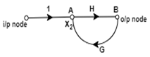
Branch: Branch is defined as a path from one node to another node, in the direction indicated by the branch arrow.

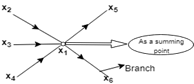
Node as a summing point:
x₁ = Summing point
x₁ =  x₂+x₃+x₄

Node as a transmitting (outgoing) point:
x₁ = x₅+x₆

Input node or source: It is the node which have only outgoing branches.
Output node or sink: It is a node which has only incoming branches.
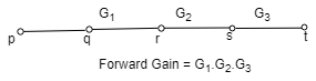
Forward Path: It is a path from an input node to an output node in the direction of branch arrow.
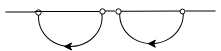
Loop: It is a path that starts and ends at the same node.

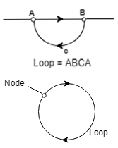
Non-touching loop: Loop is said to be non-touching if they do not have any common node.

Forward path gain: A product of all branches gain along the forward path is called Forward path gain.

Loop Gain: Loop gain is the product of branch gain which travels in the loop.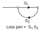

Construction of SFG and Mason Gain Formula

The SFG of a system is constructed by the following equations -

Example
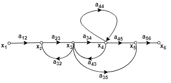
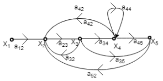
Consider a system described by following sets of equations

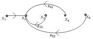
x₂ = a₂₂x₁ + a₃₂x₃ + a₄₂x₄ + a₅₂x₅

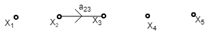
x₃ = a₂₃x₂

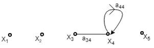
x₄ = a₃₄x₃ + a₄₄x₄

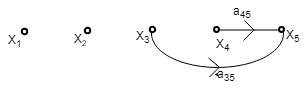
x₅ = a₃₅x₃ + a₄₅x₄

Where x1 is input and x5 is output.

Step 1 - First step is to draw all the nodes.

Step 2 - Draw the SFG for equation (1)

Step 3 - Draw the SFG for equation (2)

Step 4 - Draw the SFG for equation (3)

Step 5 - Draw the SFG for equation (4)

Step 6 - Now draw the complete signal flow graph with the help of the above graph.