Angle and Magnitude condition of root locus (with Examples) | Control Systems - Electrical Engineering (EE) PDF Download
Angle and Magnitude condition of root locus
The root locus's angle conditions help us determine whether the given point exists on the root locus branch or not. We can find the value of the system gain 'K' with the help of the magnitude condition on the root locus.
For a general closed loop system, the characteristic equation is given by:
- 1 + G(s)H(s) = 0
- G(s)H(s) = 0 - 1
- G(s)H(s) = -1
We know that the s-plane is complex. Hence, the above equation in terms of a complex variable can be written as:
- G(s)H(s) = -1 + j0
Since the s-plane is complex, G(s)H(s) is also complex. For any value of 's' to be on the root locus, it must satisfy the above equation. Both sides of the above equation are in rectangular form, and we can equate the angle and magnitude of both sides after converting them into the polar form.
The two conditions of the root locus are angle condition and magnitude condition.
Angle condition
G(s)H(s) = -1 + j0
The above equation in terms of angle can be represented as:
∠G(s)H(s) = ±(2q + 1)180º
Where,
q = 0, 1, 2 ...
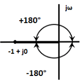
The point -1 + j0 lies on the negative real axis point, which can be traced as a magnitude one at an angle of 180 degrees, 540 degrees, ... (2q + 1)180. These values can be calculated by putting the value of q = 0, 1, 2, and so on.
For q = 0, we get 180 degrees and for q = 1, we get (2 + 1) x 180 = 540 degrees. Similarly, we can find further values.
The root locus plot of the point -1 + j0 is shown below:
 Thus, we can define the angle condition as any value of the 's' for which the root of the equation (1 + G(s)H(s) = 0) is given by:
∠G(s)H(s) = ±(2q + 1)180º
The values of the angles are the odd multiples (1, 3, 5, 7, 9 ...) of 180 degrees.
Any point on the s-plane to be on the root locus plot needs to satisfy the above condition. The angles calculated at the different values of 'q' should be the odd multiples of the positive or negative 180 degrees.
Uses of Angle condition in root locus
The common use of the angle condition in root locus is to test any point in the s-plane. It is used to find if the given point exists or not.
Magnitude condition
The magnitude condition is calculated by equating both the sides of the characteristic equation, which is given by:
1 + G(s)H(s) = 0
G(s)H(s) = -1
|G(s)H(s)| = |-1 + j0| = 1
The system gain 'K' is unknown in the magnitude condition. We cannot find the magnitude of the point at any point in the s-plane. Thus, the condition is not suitable for checking the points' existence on the root locus plot. But, if the point in the s-plane is already satisfied using the angle condition, it needs to verify the magnitude condition as well.
If the point is known to be on the root locus by the angle condition, the value of the system gain 'K' can also be found with the magnitude condition.
The magnitude condition is given by:
|G(s)H(s)| = 1
The use of the magnitude condition depends on the point on the root locus, which is verified by the angle condition.
Uses of Magnitude condition
The value of K can be determined with the help of magnitude condition, if the point is known to be on the root locus verified by the angle condition.
Example: Test whether the point -2 + 5j is present on the root locus or not. Consider the system with G(s)H(s) = K/s(s + 4).
We will first verify using the angle condition.
∠G(s)H(s) = ±(2q + 1)180º
G(s)H(s) = K/s(s + 4)
Put s = -2 + j5, we get:
= K +j0/ (-2 + j5)(-2 + j5 + 4)
= K +j0/ (-2 + j5)(2 + j5)
Converting it into polar and considering angles, we get:
- Angle G(s)H(s) = 0 /111.8 x 68.2 = -180 degrees.
- The resulted angle is the multiple of positive and negative value of 180 degrees. Thus, the angle condition is verified.
- The angle value of (-2 + 5j) = 111.8 degrees
- The angle value of (2 + 5j) = 68.2 degrees
- We can use any scientific calculator to convert from rectangular to polar.
Now, we know that the given point -2 + 5j exits on the root locus. We can use the magnitude condition, which is given by:
- |G(s)H(s)| = 1
Value of G(s)H(s) at s = -2 +5j will be:
- |K|/5.3851 X 5.3851 = 1
- After solving, K = 29
- Thus, s=-2 + 5j is one of the roots of the equation.
Graphical method to determine the value of 'K'
To determine the value of the system gain K, we need a prior knowledge of the points on the root locus, i.e., the location of the point known to be on the root locus.
The value of K is given by:
- K = product of phasor lengths drawn from the open loop poles up to a point on root locus/ product of phasor lengths drawn from the open loop zeroes up to a point on root locus
Example 1. Find the value of system gain K for the system G(s)H(s) = K/s(s + 4) Given that a point -2 + j5 is already present on the root locus plot.
We are given that a point -2 + j5 is confirmed on the root locus.
The system G(s)H(s) = K/s(s + 4) has two poles and no zeroes. It is because the numerator has no values of s.
Equating the denominator equal to zero, we get:
s(s + 4) = 0
s = 0 and s = -4
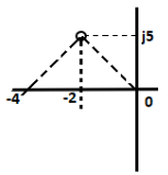
Thus, the open-loop poles are 0 and -4.
Now, we will join the points 0, -4, and -2 + j5, as shown below:Length from s = 0 to the point = pLength from s = -4 to the point = qP = (22 + 52)1/2
P = (29)1/2
Similarly, q = (22 + 52)1/2
q = (29)1/2
We know,
K = product of phasor lengths drawn from the open-loop poles up to a point on root locus/ product of phasor lengths drawn from the open-loop zeroes up to a point on root locus
Since, there is no open-loop zero, the value of the denominator will be assumed as unity.
K = p x q = 29
 Length from s = 0 to the point = pLength from s = -4 to the point = qP = (22 + 52)1/2
Example 2. To find the nature of the root locus of the given system G(s)H(s) = K/s(s + 2)
We are given a system G(s)H(s) = K/s(s + 2) has two poles and no zeroes.
We know,
1 + G(s)H(s) = 0
1 + K/s(s + 2) = 0
s(s + 2) + K = 0
s2 + 2s + K = 0
To construct the root locus for the higher-order system, we will first find the roots of the characteristic equation so formed.
s2 + 2s + K = 0
Solving the equation, we get the roots -1 + (1 - k)1/2 and -1 - (1 - k)1/2.
Now, we will find the different values of both the roots at different values ok K, which is shown in the below table:
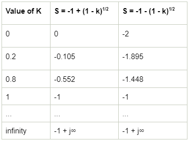
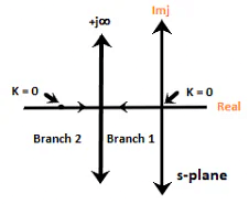
From the above table, we can conclude that there are two branches starting form 0 and -2 to infinity. The starting values 0 and -2 are also the roots of the given transfer function or the open loop poles. We can also say that the number of branches are equal to the number of open loop poles, which are two here.
|
53 videos|73 docs|40 tests
|

|
Dec 31, 2024 Last updated |

|
Explore Courses for Electrical Engineering (EE) exam
|
|
Angle and Magnitude condition of root locus (with Examples) | Control Systems - Electrical Engineering (EE)
,MCQs
,video lectures
,Angle and Magnitude condition of root locus (with Examples) | Control Systems - Electrical Engineering (EE)
,Viva Questions
,shortcuts and tricks
,Semester Notes
,practice quizzes
,Objective type Questions
,ppt
,Angle and Magnitude condition of root locus (with Examples) | Control Systems - Electrical Engineering (EE)
,Previous Year Questions with Solutions
,past year papers
,Important questions
,Sample Paper
,Summary
,Extra Questions
,mock tests for examination
,study material
,Exam
,Free
;


Angle and Magnitude condition of root locus (with Examples) Free PDF Download
Importance of Angle and Magnitude condition of root locus (with Examples)
Angle and Magnitude condition of root locus (with Examples) Notes
Angle and Magnitude condition of root locus (with Examples) Electrical Engineering (EE) Questions
Study Angle and Magnitude condition of root locus (with Examples) on the App
|
© EduRev
|
Education Revolution
|


|


within 7 days!