Rules for Sketching Root Locus (with Examples) | GATE Notes & Videos for Electrical Engineering - Electrical Engineering (EE) PDF Download
| Table of contents |
|
| Rule Number 1 |
|
| Rule Number 2 |
|
| Rule Number 3 |
|
| Rule Number 4 |
|
| Rule Number 5 |
|
| Rule Number 6 |
|
| Key Points of Sketching Root Locus |
|
| Let's Discuss an Example and use these Rules to Solve it |
|
The root locus is a graphical representation in s-domain and it is symmetrical about the real axis. Because the open loop poles and zeros exist in the s-domain having the values either as real or as complex conjugate pairs. In this document, let us discuss Rules to construct (draw) the root locus.
 Root Locus
Rule Number 1
- We know that the root of the equation can be real or complex or a combination of both. The root locus is generally symmetric about the real axis. Thus, the plot needs to be symmetric about the real axis of the s-plane.
Rule Number 2
- The transfer function of the system is generally represented by G(s)H(s), where H(s) is the feedback path. Let us suppose the open-loop transfer function to be the same G(s)H(s) and the poles and zeroes are P and Z.
- There are two conditions where the poles can be greater than the number of zeroes, or the number of zeroes can be greater than the number of poles in the given characteristic equation.
- Let the number of branches in the root locus is N. Both the cases arise when we plot the root locus. The default conditions are given for each case that helps in determining the number of branches terminating or approaching infinity.
Case 1: P > Z
- In the above case, we assume that the number of branches in the root locus will equal the number of open-loop poles. It is because the numbers of poles are greater here.
(N = P) - Branches, in this case, will start from the location of the open-loop poles. Here, out of a number of branches at P, the Z number of branches will terminate at the location of open-loop zeroes. The remaining branches (P - Z) will approach infinity.
For example,
Let P = 3, and Z = 1
Then,
The number of root locus branches = 3 = no. of poles
P - Z = 3 - 1 = 2
It means that 3 branches will start from the location of open loop poles
No. of branches terminating at the open loop zero location = 1
No. of branches approaching to infinity = P - Z = 2
Case 2: Z > P
- In the above case, we assume that the number of branches in the root locus will be equal to the number of open loop zeroes. It is because the numbers of zeroes are greater here. (N = Z)
- Branches in this case will terminate at the finite location of the open loop zeroes. Here, out of number of branches at Z, the P number of branches will start at the location of open loop poles. The remaining branches (Z - P) will approach to finite zeroes originating from the infinity.
For example,
Let P = 1, and Z = 3
Then,
The number of root locus branches = 3 = no. of zeroes
Z - P = 3 - 1 = 2
It means that 1 branch will start from the location of open loop poles
No. of branches terminating at the finite open loop pole location = 3 = all the root locus branches
No. of branches originating from infinity = Z - P = 2
Rule Number 3
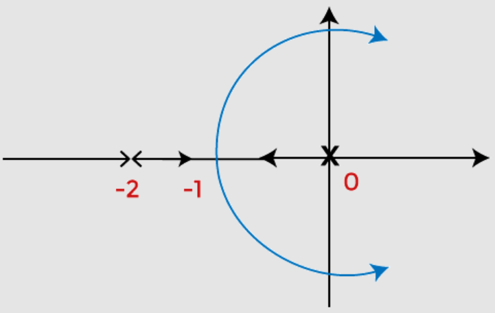
- A point on the root locus is said to exist if the sum of the open loop poles and zeroes on the real axis towards the right-hand side is odd with respect to that point.
For Example:
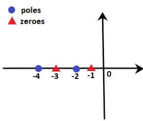
Let poles be -2 and -4, and zeroes are -1 and -3. We need to find that points -2.2 and -3.4 lies on the root locus or not.
We know that -2.2 lies between -2 and -3, while point -3.4 lies between -3 and -4. We know that -2.2 lie between -2 and -3, while point -3.4 lies between -3 and -4.
Point -2.2: At point -2.2, the sum of poles and zeroes on the right-hand side is 2, i.e. 1 pole and 1 zero. It means that the sum is even. According to rule number 3, the sum should be odd. Hence, point -2.2 does not lie on the root locus. We can also say that any point between -2 and -3 will not lie on the root locus.
Point -3.4: At point -3.4, the sum of poles and zeroes on the right-hand side is 3, i.e. 1 pole and 2 zeroes. It means that the sum is odd. According to rule number 3, the sum should be odd. Hence, point -3.4 lie on the root locus. We can also say that any point between -3 and -4 will lie on the root locus.
The area of the root locus between the points is shown below:Here, orange line represents the area where root locus lies.
 We know that -2.2 lie between -2 and -3, while point -3.4 lies between -3 and -4.
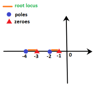 Here, orange line represents the area where root locus lies.
Example: 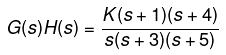 . Find on which sections of the real axis, the root locus exists.
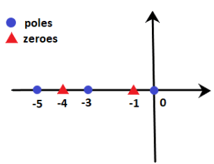
We know that the denominator signifies the poles, and the numerator signifies the zeroes. Thus, 0, -3, and -5 are the poles, and -1 and -4 are the zeroes per the given transfer function. It means that there are 3 poles and 2 zeroes.
These poles and zeroes on the real axis will appear as:
According to rule number 3:
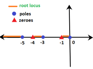
- The sections between 0 and -1 (for example, point -0.4) contain only one pole and no zeroes on the right-hand side. It means that the sum is odd (i.e. 1). So, it exists on the root locus.
- The sections between -1 and -3 (for example, point -2.1) contain only one pole and one zero on the right-hand side. It means that the sum of poles and zeroes is even (i.e. 2). So, it does not exist on the root locus.
- The sections between -3 and -4 (for example, point -3.5) contain two poles and one zero on the right-hand side. It means that the sum is odd (i.e. 3). So, it exists on the root locus.
- The sections between -4 and -3 (for example, point -4.3) contain two poles and two zeroes on the right-hand side. It means that the sum of poles and zeroes is even (i.e. 4). So, it does not exist on the root locus.
- The sections greater than -5 (for example, point -8.6) contain three poles and two zeroes on the right-hand side. It means that the sum is odd (i.e. 5). So, it exists on the root locus.
Thus, the line marked with orange depicts the sections where the root locus exists. It is shown below:
Rule Number 4
- We have already discussed that (P - Z) provides the number of branches approaching infinity for the given transfer function. The information about such branches approaching infinity is defined under rule number 4, known as asymptotes. The angle of such asymptotes is given by:
= (2q + 1)180 / P - Z
Where,
q = 0, 1, 2, 3, 4 ... (P - Z - 1)
These are always symmetric about the real axis.
Rule Number 5
- Rule number 4 describes the guidelines or information about the branches approaching infinity, known as the asymptotes. But, the angles are insufficient to plot the root locus, and the location of such branches in the s-plane is equally important, defined by rule number 5.
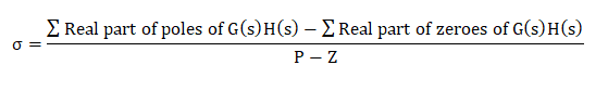
Centroid is a point where the asymptotes intersect at a common point on the real axis. It can be calculated as:

Note: The value of the centroid is always real, which can be positive or negative. It can be a part of root locus or sometimes not.
Rule Number 6
- The last rule is the breakaway point. It is also a point on the root locus where multiple roots of the given equation occurs. It is calculated for a specific value of system gain K.
Or
- It can be defined as a point on the root locus where two or more roots occur for a particular value of K.
The root locus branches always leave breakaway points at an angle of 180/n.
Where,
N = number of branches approaching at the breakaway point.
The value of the angle can be positive or negative.
Let's discuss some predictions about the existence of the breakaway points:
- There exists atleast one breakaway point between the adjacent placed poles if the section between the two poles lies on the root locus.
For example,
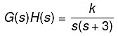
The above transfer function has two poles at 0 and -3. According to rule number 3, the point on the section between 0 and -3 (for example, point -2.2) has one pole and no zero on the right-hand side. It signifies that the sum of zeroes and poles is 1, i.e. odd. Thus, the section between 0 and -3 exists of the root locus.
Hence, there must exist a minimum of one breakaway point in between them.
Key Points of Sketching Root Locus
- Find the number of poles, zeroes, number of branches, etc., from the given transfer functions.
- Draw the plot that shows the poles and zeroes marked on it.
- Calculate the angle of asymptotes and draw a separate sketch.
- Find the centroid and draw a separate sketch.
- Find the breakaway points. These points can also be in the form of complex numbers. We can use the angle condition to verify such points in the complex form.
- Calculate the intersection points of the root locus with the imaginary axis (or y-axis).
- Calculate the angle of arrival and departure if applicable.
- Draw the final sketch of the root locus by combining all the above sketches.
- We can also predict the stability and performance of the given system using the root locus technique.
Let's Discuss an Example and use these Rules to Solve it
Example: Draw the root locus diagram for a closed loop system whose loop transfer function is given by:
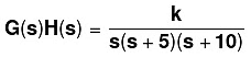
Also find if the system is stable or not.
Solution: We will follow the procedure according to the steps discussed above.
Step 1: Finding the poles, zeroes, and branches.
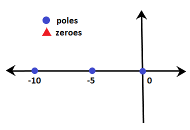
The denominator of the given transfer function signifies the poles and the numerator signifies the zeroes. Hence, there are 3 poles and no zeroes.
Poles = 0, -5, and -10
Zeroes = No zero
P - Z = 3 - 0 = 3
There are three branches (P - Z) approaching to infinity and there are no open loop zeroes. Hence infinity will be the terminating point of the root locus.
Step 2: Section of the real axis where the root locus lies.
There are three poles, which are shown below:
- The section between 0 and -5 (for example, -3.5) has only one pole on the right-hand side. It means that the sum of poles and zeroes on the side of the given point is 1.
- Rule number 3 depicts that the section between 0 and -5 lies on the root locus. Similarly, section after -10 also lies on the root locus. The section between -5 and -10 has an even number of zeroes and poles on the right-hand side. Hence, the root locus on the real axis between -5 and -10 does not exist.
- The breakaway point of the given system will lie between the section on the real axis where the root locus exists, i.e., 0 and -5.
Step 3: Angle of asymptotes.
Angle of such asymptotes is given by:
= (2q + 1)180 / P - Z
q = 0, 1, and 2
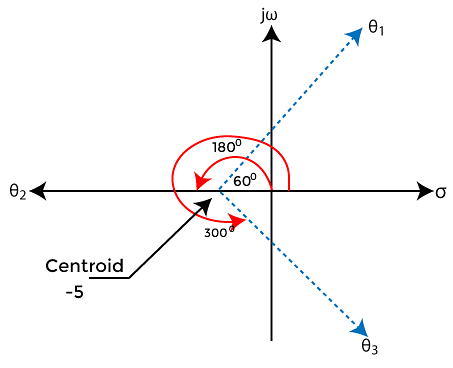
For q = 0,
Angle = 180/3 = 60 degrees
For q = 1,
Angle = 3x180/3 = 180 degrees
For q = 2,
Angle = 5x180/3 = 300 degrees
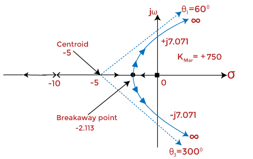
Step 4: Centroid
The centroid is given by:
= 0 - 5 - 10 - 0/3
= -15/3
= -5
Thus, the centroid of the root locus is at -5 on the real axis.
The plot showing the centroid and the angle of asymptotes is given below:
Step 5: Breakaway Point
We know that the breakaway point will lie between 0 and -5. Let's find the valid breakaway point.
1 + G(s)H(s) = 0
Putting the value of the given transfer function in the above equation, we get:
1 + K/s(s + 5)(s + 10) = 0
s(s + 5)(s + 10) + K = 0
s(s2 + 15s + 50) + K = 0
s3 + 15s2 + 50s + K = 0
K = - s3 - 15s2 - 50s
Differentiating both sides,
Dk/ds = - (3s2 + 30s + 50) = 0
3s2 + 30s + 50 = 0
Dividing the equation by 3, we get:
s2 + 10s + 16.667 = 0
Now, we will find the roots of the given equation by using the formula:
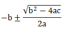
Using the value, a = 1, b = 10, and c = 16.667
The roots of the equation will be -2.113 and -7.88.
Among the two roots, only -2.113 lie between 0 and -5. Hence, it will be the breakaway point.
Let's verify by putting the value of the root in the equation K = - s3 - 15s2 - 50s.
K = - -2.113 3 - 15(-2.113)2 - 50(-2.113)
K = 48.112
The value of K is found to be positive. Thus, it is a valid breakaway point.
Step 6: Intersection with the negative real axis.
Here, we will found the intersection points of the root locus on the imaginary axis using the Routh Hurwitz criteria using the equation s3 + 15s2 + 50s + K = 0
The Routh table is shown below:
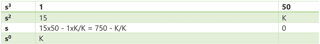
From the third rows, 750 - K/K = 0
750 - K = 0
K = 750
From the second row s2,
15 s2 + K = 0
Putting the value of Kin the above equation, we get:
15 s2 = -750
s2 = -750/15
s2 = -50
s = j7.071 and -j7.071
Both the point lies on the positive and negative imaginary axis.
Step 7: There are no complex poles present in the given transfer function. Hence, the angle of departure is not required.
Step 8: Combining all the above steps.The root locus thus formed after combining all the above steps is shown below:
Step 9: Stability of the system
The system can be stable, marginally stable, or unstable. Here, we will determine the system's stability for different values of K based on the Roth Hurwitz criteria discussed above.
The system is stable if the value of K lies between 0 and 750. The root locus at such a value of K is in the left half of the s-plane. For a value greater than 750, the system becomes unstable, and it is because the roots start moving towards the right half of the s-plane. But, at K = 750, the system is marginally stable.
We can conclude that stability is based on the location of roots in the left half or right half of the s-plane.
|
27 videos|328 docs
|
FAQs on Rules for Sketching Root Locus (with Examples) - GATE Notes & Videos for Electrical Engineering - Electrical Engineering (EE)
| 1. What are the key points to consider when sketching a root locus? |  |
| 2. How do you determine the number of branches in a root locus? | |
| 3. How do you find the breakaway and break-in points of a root locus? | |
| 4. What are the asymptotes of a root locus and how can they be determined? | |
| 5. How does the root locus cross the imaginary axis? | |

|
4.96/5 Rating |

|
Dec 22, 2024 Last updated |
|
27 videos|328 docs
|

|
Explore Courses for Electrical Engineering (EE) exam
|
|
Rules for Sketching Root Locus (with Examples) | GATE Notes & Videos for Electrical Engineering - Electrical Engineering (EE)
,Previous Year Questions with Solutions
,video lectures
,Summary
,study material
,Semester Notes
,Viva Questions
,mock tests for examination
,practice quizzes
,Exam
,Rules for Sketching Root Locus (with Examples) | GATE Notes & Videos for Electrical Engineering - Electrical Engineering (EE)
,past year papers
,Rules for Sketching Root Locus (with Examples) | GATE Notes & Videos for Electrical Engineering - Electrical Engineering (EE)
,shortcuts and tricks
,Extra Questions
,ppt
,Objective type Questions
,Sample Paper
,Important questions
,Free
,MCQs
;


Rules for Sketching Root Locus (with Examples) Free PDF Download
Importance of Rules for Sketching Root Locus (with Examples)
Rules for Sketching Root Locus (with Examples) Notes
Rules for Sketching Root Locus (with Examples) Electrical Engineering (EE) Questions
Study Rules for Sketching Root Locus (with Examples) on the App
|
© EduRev
|
Education Revolution
|


|


