Solved Examples: Root Locus | Control Systems - Electrical Engineering (EE) PDF Download

Before starting with an example, let's first discuss the steps to solve any problem on the root locus.
- Find the number of poles, zeroes, number of branches, etc., from the given transfer functions.
- Draw the plot that shows the poles and zeroes marked on it.
- Calculate the angle of asymptotes and draw a separate sketch.
- Find the centroid and draw a separate sketch.
- Find the breakaway points. These points can also be in the form of complex numbers. We can use the angle condition to verify such points in the complex form.
- Calculate the intersection points of the root locus with the imaginary axis (or y-axis).
- Calculate the angle of arrival and departure if applicable.
- Draw the final sketch of the root locus by combining all the above sketches.
- We can also predict the stability and performance of the given system using the root locus technique.
Example 1. Draw the root locus diagram for a closed loop system whose loop transfer function is given by:
G(s)H(s) = K/s(s + 5)(s + 10)
Also find if the system is stable or not.
We will follow the procedure according to the steps discussed above.
Step 1: Finding the poles, zeroes, and branches.
The denominator of the given transfer function signifies the poles and the numerator signifies the zeroes. Hence, there are 3 poles and no zeroes.
Poles = 0, -5, and -10
Zeroes = No zero
P - Z = 3 - 0 = 3
There are three branches (P - Z) approaching to infinity and there are no open loop zeroes. Hence infinity will be the terminating point of the root locus.
Step 2: Section of the real axis where the root locus lies.
There are three poles, which are shown below:
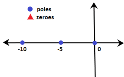
The section between 0 and -5 (for example, -3.5) has only one pole on the right-hand side. It means that the sum of poles and zeroes on the side of the given point is 1. Rule number 3 depicts that the section between 0 and -5 lies on the root locus. Similarly, section after -10 also lies on the root locus. The section between -5 and -10 has an even number of zeroes and poles on the right-hand side. Hence, the root locus on the real axis between -5 and -10 does not exist. The breakaway point of the given system will lie between the section on the real axis where the root locus exists, i.e., 0 and -5.
Step 3: Angle of asymptotes.
Angle of such asymptotes is given by:
= (2q + 1)180 / P - Z
q = 0, 1, and 2
For q = 0,
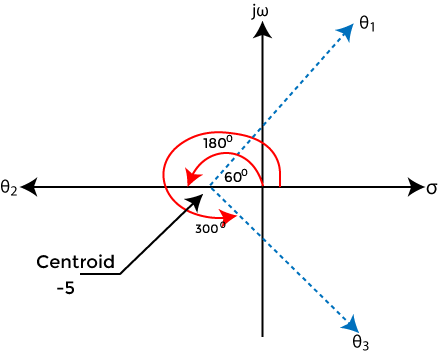
Angle = 180/3 = 60 degrees
For q = 1,
Angle = 3x180/3 = 180 degrees
For q = 2,
Angle = 5x180/3 = 300 degrees
Step 4: Centroid
The centroid is given by: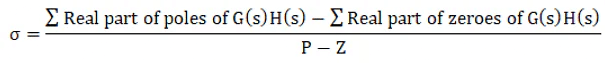
= 0 - 5 - 10 - 0/3= -15/3
= -5
Thus, the centroid of the root locus is at -5 on the real axis.
The plot showing the centroid and the angle of asymptotes is given below:
Step 5: Breakaway point
We know that the breakaway point will lie between 0 and -5. Let's find the valid breakaway point.
1 + G(s)H(s) = 0
Putting the value of the given transfer function in the above equation, we get:
1 + K/s(s + 5)(s + 10) = 0
s(s + 5)(s + 10) + K = 0
s(s2 + 15s + 50) + K = 0
s3 + 15s2 + 50s + K = 0
K = - s3 - 15s2 - 50s
Differentiating both sides,
Dk/ds = - (3s2 + 30s + 50) = 0
3s2 + 30s + 50 = 0
Dividing the equation by 3, we get:
s2 + 10s + 16.667 = 0
Now, we will find the roots of the given equation by using the formula:
Using the value, a = 1, b = 10, and c = 16.667
The roots of the equation will be -2.113 and -7.88.
Among the two roots, only -2.113 lie between 0 and -5. Hence, it will be the breakaway point.
Let's verify by putting the value of the root in the equation K = - s3 - 15s2 - 50s.
K = - -2.113 3 - 15(-2.113)2 - 50(-2.113)
K = 48.112
The value of K is found to be positive. Thus, it is a valid breakaway point.
Step 6: Intersection with the negative real axis.
Here, we will found the intersection points of the root locus on the imaginary axis using the Routh Hurwitz criteria using the equation s3 + 15s2 + 50s + K = 0
The Roth table is shown below: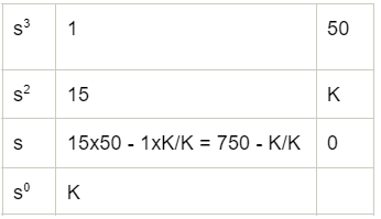
From the third row s, 750 - K/K = 0
750 - K = 0
K = 750
From the second row s2,
15 s2 + K = 0
Putting the value of Kin the above equation, we get:
15 s2 = -750
s2 = -750/15
s2 = -50
s = j7.071 and -j7.071
Both the point lies on the positive and negative imaginary axis.
Step 7: There are no complex poles present in the given transfer function. Hence, the angle of departure is not required.
Step 8: Combining all the above steps.
The root locus thus formed after combining all the above steps is shown below: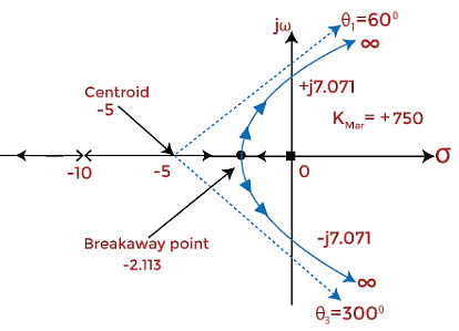
Step 9: Stability of the system
- The system can be stable, marginally stable, or unstable. Here, we will determine the system's stability for different values of K based on the Roth Hurwitz criteria discussed above.
- The system is stable if the value of K lies between 0 and 750. The root locus at such a value of K is in the left half of the s-plane. For a value greater than 750, the system becomes unstable, and it is because the roots start moving towards the right half of the s-plane. But, at K = 750, the system is marginally stable.
- We can conclude that stability is based on the location of roots in the left half or right half of the s-plane.
Impact of the addition of pole and zero on the root locus
Impact of the addition of pole
The impact of the adding pole to the left half of the s-plane will push the root locus towards the right side of the s-plane. We know that the system tends to be stable when the roots lie on the left half of the s-plane. When the root locus moves towards right half, the stability reduces. It means that the addition of pole on the root locus will decrease the stability of the system. The range of 'K' and the gain margin f the system also decreases.
For example,
Consider the plot of the system G(s)H(s) = K/s(s + 2)(s + 4).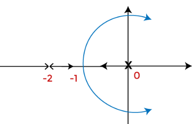 Now, let's add s = -6 pole to the above system. The root locus plot will now appear as:
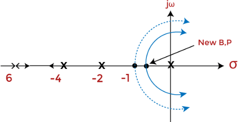
G(s)H(s) = K/s(s + 2)(s + 4)(s + 6).
We can notice that the addition of pole resulted in the root locus too shift towards the right-half of the s-plane.
Impact of the addition of zero
- The impact of the adding zero will push the root locus towards the left side of the s-plane. We know that the system tends to be stable when the roots lie on the left half of the s-plane. When the root locus moves towards left half, the stability improves. It means that the addition of zero on the root locus will increase the stability of the system. The range of 'K' and the gain margin f the system also increases. Here, the root locus will shift towards the added zero.
For example,
Consider the system G(s)H(s) = K(s + 4)/s(s + 2).
Now, let's add zero s = -6 to the above system. The root locus plot will now appear as: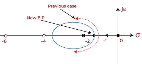 G(s)H(s) = K(s + 4)(s + 6)/s(s + 2).
We can notice that the addition of pole resulted in the root locus too shift towards the right-half of the s-plane.
|
53 videos|107 docs|40 tests
|


shortcuts and tricks
,Summary
,ppt
,Solved Examples: Root Locus | Control Systems - Electrical Engineering (EE)
,video lectures
,Semester Notes
,MCQs
,Previous Year Questions with Solutions
,Objective type Questions
,Free
,Important questions
,Exam
,mock tests for examination
,practice quizzes
,Viva Questions
,past year papers
,Solved Examples: Root Locus | Control Systems - Electrical Engineering (EE)
,Extra Questions
,Sample Paper
,Solved Examples: Root Locus | Control Systems - Electrical Engineering (EE)
,study material
;


Solved Examples: Root Locus Free PDF Download
Importance of Solved Examples: Root Locus
Solved Examples: Root Locus Notes
Solved Examples: Root Locus Electrical Engineering (EE) Questions
Study Solved Examples: Root Locus on the App
|
© EduRev
|
Education Revolution
|


|


