Controllability & Observability | Control Systems - Electrical Engineering (EE) PDF Download

Controllability

If the state of the system can be transferred to another desired state over a finite time period by using input is called controllability.
Consider the state equations
y(t) = C x(t) + D u(t)
where x denotes the state variable
u denotes the input variable
y denotes the output variable.
Kalman’s Test for Controllability
If a system matrix A has order n × n
Then we form a controllability matrix (Qc)
Qc = [B : AB : A2B : A3B : ……………… : An-2B : An-1B]
where controlled matrix B must be a column matrix.
The order of Qc is n × n.
Case-1: The system is controllable if the rank of Qc is ‘n’. In other words, when the determinant of Qc is non-zero, the system is controllable i.e. |Qc| ≠ 0.
Case-2: If |Qc| = 0 or the rank of Qc is not equal to ‘n’ then the system is said to be uncontrollable.
In order to check how many states are controllable in case-2, we consider sub-matrices of Qc of order (n-1) × (n-1) and again compute the determinant.
(i) If the determinant of any submatrices is non-zero then the rank will be (n-1). Hence the number of controllable states will be (n – 1).
(ii) If the determinant of all submatrices is zero then we consider sub-matrices of Qc of order (n-2) × (n-2) and again compute the determinant. If the determinant of any submatrices is non-zero then the rank will be (n-2). Hence the number of controllable states will be (n – 2).
The above steps are followed in a similar fashion until we get a non-zero determinant of any submatrices.

Gilbert’s Test to check controllability

It states that
A system is said to be controllable if row of B corresponding to the last row of each Jordan Block is non-zero.
A system is said to be controllable if all rows of B is non-zero in case matrix A is in diagonal canonical form.
Gilbert’s test is only applicable if matrix A is in Jordan canonical form or Diagonal canonical form.
Let us understand with the help of an example of Jordan canonical form.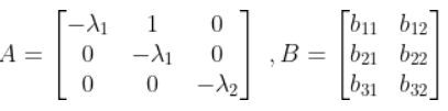
Here matrix A is in Jordan canonical form. The Jordan block JB₁ and JB₂ are
To check controllability, we see the last row of Jordan blocks.
The last row of Jordan block JB₁ corresponds to the second row of matrix A. The last row of Jordan block JB₂  corresponds to the third row of matrix A.
Hence according to Gilbert’s test, we check the corresponding second and third rows of matrix B.
If these second and third rows of matrix B are non-zero then the system is controllable.
Let us understand with the help of an example of Diagonal canonical form.
Now we treat it as Jordan canonical form with each Jordan block of order 1 × 1.
The Jordan block JB₁, JB₂ and JB₃ are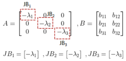
To check controllability, we see the last row of Jordan blocks.

• The last row of Jordan block JB₁ corresponds to the first row of matrix A.
• The last row of Jordan block JB₂ corresponds to the second row of matrix A.
• The last row of Jordan block JB₃ corresponds to the third row of matrix A.

Hence according to Gilbert’s test, we check the corresponding first, second, and third rows of matrix B.
If these first, second, and third rows of matrix B are non-zero then the system is controllable.

Observability

If all states of the system can be determined from the knowledge of output of the system at a given time is called observability.

Kalman’s Test for Observability

If a system matrix A has order n × n
Then we form an observability matrix (Q_o)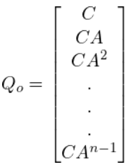

Here, output matrix C is a row matrix.
The order of Q_o is n × n.
Case-1: The system is observable if the rank of Q_o is ‘n’. In other words, when the determinant of Qo is non-zero, the system is observable i.e. |Q_o| ≠ 0.
Case-2: If |Q_o| = 0 or the rank of Q_o is not equal to ‘n’ then the system is said to be unobservable.
In order to check how many states are observable in case-2, we consider sub-matrices of Q_o of order (n-1) × (n-1) and again compute the determinant.
(i) If the determinant of any submatrices is non-zero then the rank will be (n-1). Hence the number of observable states will be (n – 1).
(ii) If the determinant of all submatrices is zero then we consider sub-matrices of Qo of order (n-2) × (n-2) and again compute the determinant. If the determinant of any submatrices is non-zero then the rank will be (n-2). Hence the number of observable states will be (n – 2).
The above steps are followed in a similar fashion until we get a non-zero determinant of any submatrices.

Gilbert’s Test to check observability

It states that
A system is said to be observable if columns of C corresponding to the first row of each Jordan Block is non-zero.
A system is said to be observable if all columns of C is non-zero in case matrix A is in diagonal canonical form.
Gilbert’s test is only applicable if matrix A is in Jordan canonical form or Diagonal canonical form.
Let us understand with the help of an example of Jordan canonical form.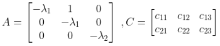
Here matrix A is in Jordan canonical form. The Jordan block JB₁ and JB₂ are
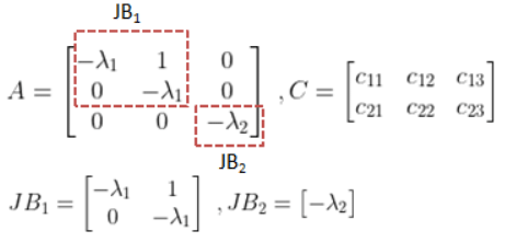To check observability, we see the first row of Jordan blocks.

• The first row of Jordan block JB₁ corresponds to the first row of matrix A.
  The first row of Jordan block JB₂ corresponds to the third row of matrix A.

Hence according to Gilbert’s test, we check the corresponding first and third columns of matrix C.
If these first and third columns of matrix C are non-zero then the system is unobservable.
Let us understand with the help of an example of Diagonal canonical form.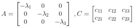
Now we treat it as Jordan canonical form with each Jordan block of order 1 × 1.
The Jordan block JB₁, JB₂ and JB₃ are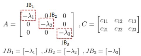
To check observability, we see the first row of Jordan blocks.

• The first row of Jordan block JB1 corresponds to the first row of matrix A.
• The first row of Jordan block JB2 corresponds to the second row of matrix A.
• The first row of Jordan block JB3 corresponds to the third row of matrix A.

Hence according to Gilbert’s test, we check the corresponding first, second, and third columns of matrix C.
If these first, second, and third columns of matrix C are non-zero then the system is observable.