Taylor Series | Engineering Mathematics - Engineering Mathematics PDF Download

Taylor series is the polynomial or a function of an infinite sum of terms. Each successive term will have a larger exponent or higher degree than the preceding term.

The above Taylor series expansion is given for a real values function f(x) where f’(a), f’’(a), f’’’(a), etc., denotes the derivative of the function at point a. If the value of point ‘a’ is zero, then the Taylor series is also called the Maclaurin series.

Taylor’s Series Theorem

Assume that if f(x) be a real or composite function, which is a differentiable function of a neighbourhood number that is also real or composite. Then, the Taylor series describes the following power series :

In terms of sigma notation, the Taylor series can be written as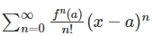

Where
f⁽ⁿ⁾ (a) = n^th derivative of f
n! = factorial of n.

Proof

We know that the power series can be defined as

When x = 0,
f(x)= a₀ 
So, differentiate the given function, it becomes,
f’(x) = a₁+ 2a₂x + 3a₃x² + 4a₄x³ +….
Again, when you substitute x = 0, we get
f’(0) =a₁
So, differentiate it again, we get
f”(x) = 2a₂ + 6a₃x +12a₄x² + …
Now, substitute x=0 in second-order differentiation, we get

f”(0) = 2a₂
Therefore, [f”(0)/2!] = a₂
By generalising the equation, we get
f ⁿ (0) / n! = a_n
Now substitute the values in the power series we get,

Generalise f in more general form, it becomes
f(x) = b + b₁ (x-a) + b₂( x-a)² + b₃ (x-a)³+ ….
Now, x = a, we get
b_n = fⁿ(a) / n!
Now, substitute b_n in a generalised form

Hence, the Taylor series is proved.

Taylor Series of Sin x

f(x) = sin x
f’(x) = cos x
f’’(x) = -sin x
f’’’(x) = -cos x
f’’’’(x) = sin x
And so on
The taylor series for Sin x at x = 0, is given by: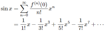

Taylor Series in Several Variables

The Taylor series is also represented in the form of functions of several variables. The general form of the Taylor series in several variables is

Maclaurin Series

If the Taylor Series is centred at 0, then the series is known as the Maclaurin series. It means that,
If a= 0 in the Taylor series, then we get;

This is known as the Maclaurin series.
Example: Maclaurin series of 1/(1-x) is given by:
1+x+x²+x³+x⁴+…, 

Applications of Taylor Series

The uses of the Taylor series are:

• Taylor series is used to evaluate the value of a whole function in each point if the functional values and derivatives are identified at a single point.
• The representation of Taylor series reduces many mathematical proofs.
• The sum of partial series can be used as an approximation of the whole series.
• Multivariate Taylor series is used in many optimization techniques.
• This series is used in the power flow analysis of electrical power systems.

Problems and Solutions

Question 1: Determine the Taylor series at x=0 for f(x) = e^x 

Given: f(x) = e^x
Differentiate the given equation,
f’(x) = e^x
f’’(x) =e^x
f’’’(x) = e^x
At x=0, we get
f’(0) = e⁰ =1
f’’(0) = e⁰=1
f’’’(0) = e⁰ = 1
When Taylor series at x= 0, then the Maclaurin series is

e^x = 1+ x(1) + (x²/2!)(1) + (x³/3!)(1) + ….. 
Therefore, e^x = 1+ x + (x²/2!) + (x³/3!)+ …..

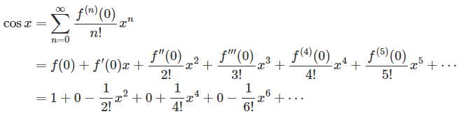
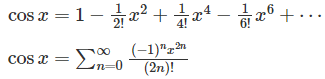
Question 2: EValuate the Taylor Series for  f ( x ) = cos ( x )  for  x = 0.

We need to take the derivatives of the cos x and evaluate them at  x = 0.
f(x) = cos x  ⇒ f(0) = 1
f’(x) = -sin x ⇒ f’(0) = 0
f’’(x) = -cos x ⇒ f’’(0) = -1
f’’’(x) = sin x ⇒ f’’’(0) = 0
f’’’’(x) = cos x ⇒ f’’’’(4) = 1
f(5)(x) = -sin x ⇒ f(5) (0) = 0
f(6) (x) = -cos x ⇒ f(6)(0) = -1
Therefore, according to the Taylor series expansion;

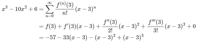
Question 3: Evaluate the Taylor Series for  f (x) = x³ − 10x² + 6  at  x = 3. 

First, we will find the derivatives of the given function.
f(x) =  x³ − 10x² + 6 ⇒ f(3) = -57
f’(x) = 3x² − 20x ⇒ f’(3) = 33
f’’(x) = 6x – 20 ⇒ f’’(3) = -2
f’’’(x) = 6 ⇒ f’’’(3) = 6
f’’’’(x) = 0 
Therefore, the required series is: