Named Ranges in Excel | How to become an Expert of MS Excel - Class 6 PDF Download
| Table of contents |

|
| Introduction |

|
| What are Named Ranges? |

|
| Creating Named Ranges |

|
| Using Named Ranges |

|
| Examples and Code Explanation |

|
| Sample Problems with Solutions |

|
Introduction
Excel is a powerful tool for organizing and analyzing data, and one of its most useful features is the ability to create named ranges. Named ranges allow you to assign a meaningful name to a specific cell or range of cells, making it easier to reference and work with data in your spreadsheets. In this article, we will explore the concept of named ranges, learn how to create and use them, and provide practical examples to reinforce your understanding.
What are Named Ranges?
Named ranges are user-defined labels or names assigned to specific cells or ranges in an Excel worksheet. Instead of using cell references (such as A1 or B2:C10) in formulas or functions, you can use the names you assign to these ranges. This not only makes your formulas easier to understand but also improves the readability and maintainability of your spreadsheets.
Creating Named Ranges
Creating named ranges is straightforward in Excel. Here's how you can do it:
- Select the cell or range of cells you want to name.
- Go to the "Formulas" tab in the Excel ribbon.
- Click on the "Define Name" button in the "Defined Names" group.
- In the "New Name" dialog box, enter a name for your range (avoid using spaces or special characters).
- Choose the scope for the named range (Workbook or Worksheet).
- Verify the cell reference in the "Refers to" field, or manually enter the desired range.
- Click "OK" to create the named range.
Using Named Ranges
Once you have created named ranges, you can utilize them in various ways throughout your Excel workbook:
- In formulas: Instead of referencing individual cells or ranges by their cell references, you can simply use the assigned names. For example, instead of "=A1+B1," you can write "=Sales+Expenses," assuming "Sales" and "Expenses" are your named ranges.
- Data validation: Named ranges are handy when setting up data validation rules. You can use them as the source for dropdown lists or restrict input to specific ranges.
- Conditional formatting: Apply conditional formatting rules based on named ranges. For instance, highlight cells in a named range "HighPriority" with a specific format when their values exceed a certain threshold.
- Charts and graphs: When creating charts or graphs, you can refer to named ranges for your data series or axis labels. This simplifies the process of updating your charts when new data is added.
Examples and Code Explanation
Let's dive into some examples to better understand how named ranges work.
Example 1: Basic Calculation
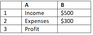
Consider a simple budget spreadsheet with the following data:
Instead of manually entering formulas like "=B1-B2" for profit, let's create named ranges.
- Select cell B1 and name it "Income."
- Select cell B2 and name it "Expenses."
Now, in cell B3, you can enter the formula "=Income-Expenses" to calculate the profit. Whenever you update the values in the "Income" or "Expenses" cells, the profit will automatically recalculate.
Example 2: Data Validation
Suppose you have a list of products in column A, and you want to restrict the input in cell B1 to the products in the list.
- Select the range A1:A5 and name it "ProductList."
- Go to cell B1 and choose "Data Validation" from the "Data" tab.
- In the settings, select "List" as the validation criteria.
- In the "Source" field, enter "=ProductList" (without quotes).
Now, cell B1 will have a dropdown list containing the products from the "ProductList" named range, ensuring valid input.
Sample Problems with Solutions
Problem 1: Calculate the average sales from a range named "SalesData" (A1:A10).
Enter the formula "=AVERAGE(SalesData)" in the desired cell.
Problem 2: Apply conditional formatting to highlight cells in the range named "Inventory" (B2:F10) if the value exceeds 100.
- Select the range B2:F10.
- Choose "Conditional Formatting" from the "Home" tab.
- Select "New Rule" and choose "Use a formula to determine which cells to format."
- Enter the formula "=Inventory>100" (without quotes).
- Choose the desired format and click "OK."
Conclusion
Named ranges are powerful tools in Excel that enhance the readability, usability, and maintainability of your spreadsheets. By assigning meaningful names to cells or ranges, you can simplify formulas, improve data validation, and streamline chart creation. Experiment with named ranges in your own spreadsheets to unlock their full potential and make your Excel experience even more productive.
|
92 videos|62 docs|15 tests
|


