Creating a Pivot Table in Excel | How to become an Expert of MS Excel - Class 6 PDF Download
| Table of contents |

|
| Introduction |

|
| What is a Pivot Table? |

|
| How to Create a Pivot Table in Excel |

|
| Pivot Table Example 1: Sales Data |

|
| Pivot Table Example 2: Survey Results |

|
| Sample Problems with Solutions |

|
Introduction
Excel is a powerful tool that allows you to analyze and summarize data efficiently. One of the key features in Excel is the Pivot Table, which enables you to transform a large set of data into a more manageable and insightful format. In this article, we will guide you through the process of creating a Pivot Table in Excel, step by step, with multiple examples and simple codes.
What is a Pivot Table?
A Pivot Table is a data summarization tool in Excel that allows you to extract meaningful insights from large datasets. It enables you to reorganize, filter, and analyze your data based on different criteria, such as categories, dates, or numerical values. Pivot Tables offer a flexible and dynamic way to view and understand your data, making it easier to identify trends, patterns, and relationships.
How to Create a Pivot Table in Excel
Preparing Your Data
Before creating a Pivot Table, it's essential to ensure that your data is well-structured and organized. Follow these best practices:
- Place each data category in a separate column.
- Use headers for your columns.
- Remove any blank rows or columns.
- Ensure consistent data formatting.
Creating a Pivot Table
Now, let's create a Pivot Table using the following steps:
Step 1: Select your data: Highlight the range of cells that contain your data.
Step 2: Insert a Pivot Table: Go to the "Insert" tab in the Excel ribbon, and click on the "PivotTable" button. A dialog box will appear.
Step 3: Choose your data source: Ensure that the "Select a table or range" option is selected in the dialog box. The correct range should be automatically populated. Click "OK" to proceed.
Step 4: Designate the Pivot Table destination: Choose where you want your Pivot Table to be placed. You can select either a new worksheet or an existing one.
Step 5: Customize your Pivot Table: A Pivot Table Field List will appear on the right side of your Excel window. Drag and drop the desired fields into the "Row Labels," "Column Labels," and "Values" areas based on how you want your data to be organized and summarized.
Step 6: Analyze your data: Excel will generate a basic Pivot Table based on your selections. You can further customize it by adding filters, calculations, and sorting options.
Modifying a Pivot Table
If you need to make changes to your Pivot Table, follow these steps:
- To add or remove fields: Simply drag and drop them from or to the Field List.
- To change the summary calculation: Click on the drop-down arrow next to the value field in the Pivot Table and choose a different summary function (e.g., sum, count, average).
- To filter data: Click on the drop-down arrow next to the field you want to filter and select the desired criteria.
- To sort data: Click on the drop-down arrow next to the field you want to sort and choose the desired sorting order.
Pivot Table Example 1: Sales Data
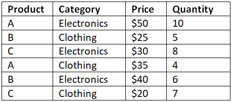
Let's consider a sample dataset of sales records to demonstrate the use of Pivot Tables.
By creating a Pivot Table, you can quickly summarize this data and gain insights.
Code:
- Select the range of data and go to the "Insert" tab.
- Click on the "PivotTable" button.
- In the dialog box, ensure the correct range is selected and choose the destination.
- Drag the "Product" field to the "Row Labels" area.
- Drag the "Category" field to the "Column Labels" area.
- Drag the "Price" field to the "Values" area and choose the summary function as "Sum."
- Drag the "Quantity" field to the "Values" area and choose the summary function as "Sum."
Output:
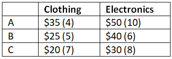
A Pivot Table will be created, summarizing the sales data as follows:
This Pivot Table provides a clear overview of the total sales and quantity for each product and category.
Pivot Table Example 2: Survey Results
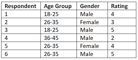
Now, let's explore another example using survey data. We can create a Pivot Table to analyze the survey results.
Code:
- Select the range of data and go to the "Insert" tab.
- Click on the "PivotTable" button.
- In the dialog box, ensure the correct range is selected and choose the destination.
- Drag the "Age Group" field to the "Row Labels" area.
- Drag the "Gender" field to the "Column Labels" area.
- Drag the "Rating" field to the "Values" area and choose the summary function as "Average."
Output:
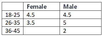
A Pivot Table will be created, summarizing the survey results as follows: This Pivot Table allows us to compare the average ratings given by respondents across different age groups and genders.
Sample Problems with Solutions
Problem 1: Create a Pivot Table to summarize the total sales quantity for each product category.
Code:
- Select the range of data and go to the "Insert" tab.
- Click on the "PivotTable" button.
- In the dialog box, ensure the correct range is selected and choose the destination.
- Drag the "Category" field to the "Row Labels" area.
- Drag the "Quantity" field to the "Values" area and choose the summary function as "Sum."
Output:
A Pivot Table will be created, summarizing the total sales quantity for each product category.
Problem 2: Create a Pivot Table to analyze the average ratings given by respondents for each age group and gender combination.
Code:
- Select the range of data and go to the "Insert" tab.
- Click on the "PivotTable" button.
- In the dialog box, ensure the correct range is selected and choose the destination.
- Drag the "Age Group" field to the "Row Labels" area.
- Drag the "Gender" field to the "Column Labels" area.
- Drag the "Rating" field to the "Values" area and choose the summary function as "Average."
Output:
A Pivot Table will be created, summarizing the average ratings for each age group and gender combination.
Conclusion
Pivot Tables are an invaluable tool for analyzing and summarizing large datasets in Excel. They allow you to transform raw data into meaningful insights, providing a clear understanding of patterns, trends, and relationships. By following the steps outlined in this article and exploring the provided examples, you can start leveraging the power of Pivot Tables to enhance your data analysis skills.
|
92 videos|62 docs|15 tests
|


