Graphs: Motion in One Dimension | AP Physics 1 - Grade 9 PDF Download
| Table of contents |
|
| Analysis of Motion through Graphs |
|
| Displacement–Time Graph |
|
| Velocity–Time Graph |
|
| Acceleration–Time Graph |
|

Analysis of Motion through Graphs
Let us see some basics points of graphs before analyzing the motion of an object through graphs.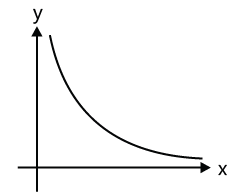 Basic Graphs: (a) A linear relationship between x and y represents a straight line.
E.g., y= 4x - 2, y= 5x + 3, 3x = y - 2
(b) A proportionality relationship between x and y (i.e. x ∝ y or y = kx ) represents a straight line passing through origin.
(c) Inverse proportionality (x ∝ 1/y) or xy=k represents a rectangular hyperbola.
Shape of a rectangular hyperbola is given in the graph:
(d) A quadratic equation in x and y represents a parabola in x-y graph. E.g., y = 3x2 +2, y2 = 4x, x2 = y-2
Analysis of Graphs: (a) If z dy/dx, the value of z at any point on x-y graph can be obtained by the slope of the graph at that point.
(b) If z = y(dx) or x(dy), the value of z between x1 and x2 or y1 and y2 is obtained by the area of graph between x1 and x2 or y1 and y2.
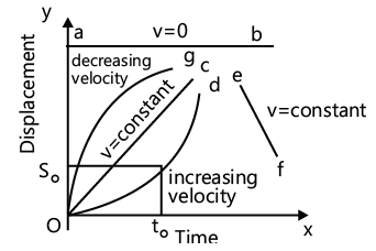
Displacement–Time Graph
With displacement of a body plotted on y-axis against time on x-axis, displacement–time curve is obtained.
(a) The slope of the tangent at any point of time gives the instantaneous velocity at any given instant.
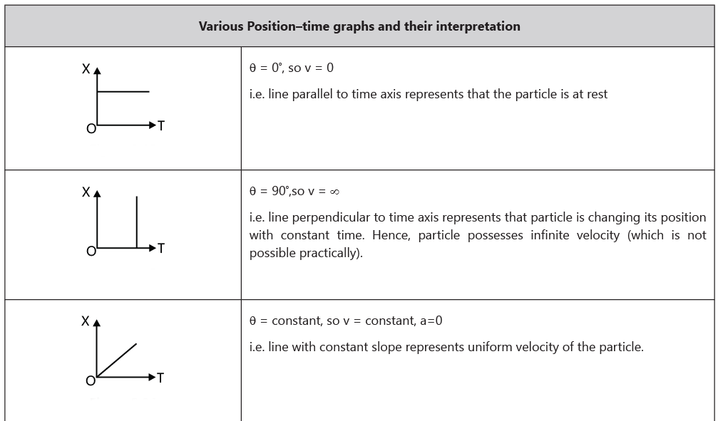
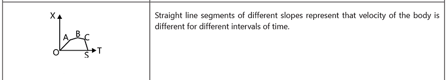
(b) At a uniform motion the displacement–time graph is a straight line.
- If the graph obtained is parallel to time axis, the velocity is zero.
- If the graph is an oblique line, the velocity is constant (OC and EF in Fig. 2).
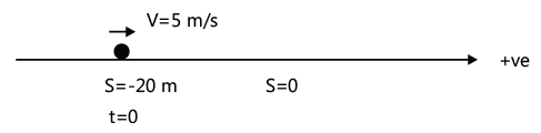
Example: Displacement–time graph of a particle moving in a straight line is shown in the Fig. State whether the motion is accelerated or not. Describe the motion of the particle in detail. Given s0=20 m and t0=4 s.
 Solution: The velocity of the particle at any instant is the slope of the displacement time graph at that instant. If the slope is constant, velocity is constant.
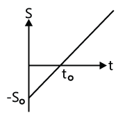
Slope s–t is a straight line. Hence, velocity of particle is constant. At time t = 0, displacement of the particle from its mean position is –s0 i.e. -20 m. Velocity of particle, V slope s0/t0 = 20/4 = 5m / s
At t = 0 particle is at –20 m and has a constant velocity of 5 m/s. At t0 = 4 sec, particle will pass through its mean position
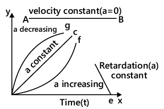
Velocity–Time Graph
Displacement, velocity and acceleration, specifying the entire motion, can be determined by the velocity–time curve.
- Instantaneous acceleration can be obtained by the slope of the tangent at any point corresponding to a particular time on the curve.
- Displacement during a time interval is obtained from the area enclosed by velocity–time graph and time axis for a time interval.
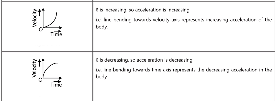
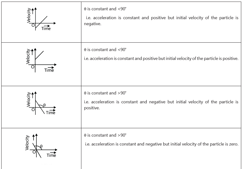
- For a uniformly accelerated motion, velocity–time graph is a straight line.
- For constant velocity (i.e. acceleration is zero), the graph obtained is a straight line AB parallel to x-axis (time).
- For constant acceleration, the graph obtained is oblique.
Acceleration–Time Graph
- Change in velocity for a given time interval is the area enclosed between acceleration–time graph and time axis.
- For constant acceleration, the obtained graph is a straight line parallel to x-axis, i.e. time (t).
- If the acceleration is non-uniform, then the graph is oblique.
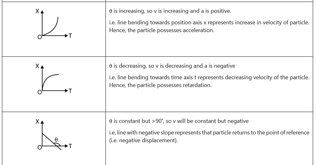
Inference: Displacement–time graph for uniformly accelerated or retarded motion is a parabola. Since, for constant acceleration, then relation between displacement and time is: s = ut ± 1/2at2 which is quadratic in nature. Thus, displacement–time graph will be parabolic in nature.
Example: Acceleration–time graph of a particle moving in a straight line is shown in Fig. At time t=0, velocity of the particle is 2 m/s. Find velocity at the end of the 4th second.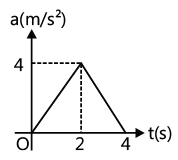 Solution: The area enclosed by the acceleration-time graph between t = 0 and t = 4s will give the change in velocity in this time interval.
dv = a dt
or change in velocity = area under a-t graph
Hence vf - vi = 1/2 (4) (4) = 8m/s; ∴ vf - vi + 8 = (2 + 8)m/ s = 10m/ s
The following are the lists of motions that are not possible practically:
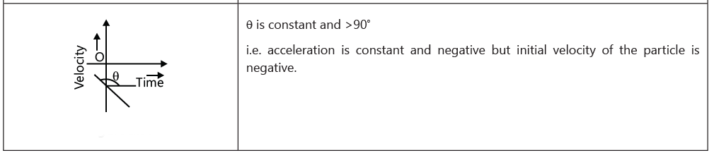
- Slopes of v-t or s-t graphs can never be infinite at any point, because infinite slope of v-t graph means infinite acceleration. Similarly, infinite slope of s-t graph means infinite velocity. Hence, the graphs shown here are not possible.
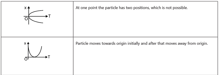
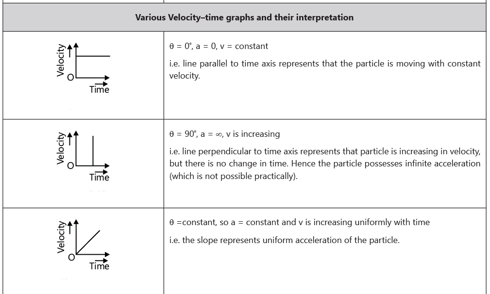
- At a particular time, two values of velocities v1 and v2 or displacements S1 and S2 are not possible. Hence, the following graphs shown here are not possible.
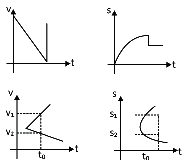
Example 1: At t = 0, a particle is at rest at origin. For the first 3 s the acceleration is 2 ms-2 and for the next 3 s acceleration is -2 ms-2. Find the acceleration versus time, velocity versus time and position versus time graphs.
Solution: The area enclosed by the acceleration-time graph and the time-axis between t = 0 and t = t gives the change in velocity in this time interval. Similarly the area enclosed by the velocity-time graph and the time-axis between t = 0 and t = t will give the change in displacement in this time interval. Given for the first 3 s acceleration is 2 ms-2 and for next 3 s acceleration is -2 ms-2. Hence acceleration-time graph is as shown in the Fig.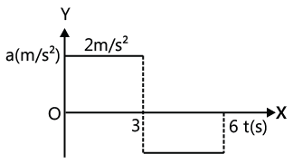 The area enclosed between a-t curve and t-axis gives change in velocity for the corresponding interval. Also at t = 0, v = 0, hence final velocity at t = 3 s will increase to 6 ms-1. In next 3 s the velocity will decrease to zero. Hence the velocity-time graph is as shown in figure.
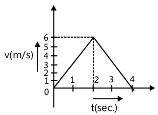 Note that due to constant acceleration v-t curves are taken as straight line.
Now for x-t curve, we will use the fact that area enclosed between v-t curve and time axis gives displacement for the corresponding interval. Hence displacement in the first 3 s is 4.5 m and in next 3 s is 4.5 m. Also the x–t curve will be of parabolic nature as the motion has a constant acceleration. Therefore, x–t curve is as shown in figure.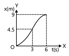
Example 2: The graph in the Fig. shows the velocity of a body plotted as a function of time.
(a) Find the instantaneous acceleration at t = 3 s, 7 s, 10 s, and 13 s.
(b) Find the distance travelled by the body in the first 5 s, 9 s, and 14 s
(c) Find the total distance covered by the body during motion.
(d) Find the average velocity of the body during motion.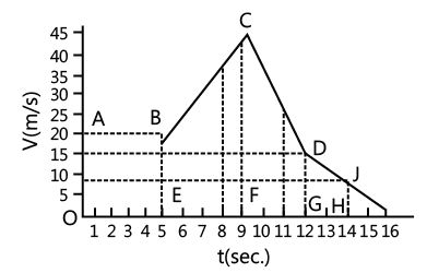
Solution: The area enclosed by the acceleration-time graph and the time-axis between t = 0 and t = t gives the change in velocity in this time interval. Similarly the area enclosed by the velocity-time graph and the time-axis between t = 0 and t = t will give the change in displacement in this time interval.
(a) Acceleration at t = 3 s
When the particle travels from point A to B for the first 5 s, the body moves with a constant velocity. Hence, the acceleration is zero.
Acceleration at t = 7 s.
When the particle travels from point B to C for the interval 5 to 9 s, the acceleration is uniform.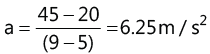
Hence acceleration at t=7 s is 6.25 m/s2. The acceleration at t = 10 s and 13 s are respectively -10 m/s2 and -3.75 m.s2.
(b) The distance covered in t seconds is the area enclosed by the curve in t seconds on velocity–time graph. The distance covered by the body in 5 s = Area of rectangle ABEO = 20 x 5 = 100 m
The distance covered in first 9 s = The area of the figure ABCFO = Area ABEO + Area EBCF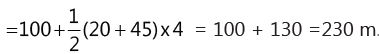
The distance covered by the body in first 14 s = Area [(ABCFO) + (CDGF) + DJHG)]
(c) The distance covered by the body during the entire motion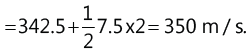
(d) Average velocity for the motion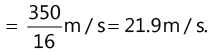
|
48 videos|69 docs|30 tests
|


study material
,Extra Questions
,video lectures
,MCQs
,Sample Paper
,Graphs: Motion in One Dimension | AP Physics 1 - Grade 9
,Summary
,Free
,shortcuts and tricks
,Previous Year Questions with Solutions
,Exam
,Graphs: Motion in One Dimension | AP Physics 1 - Grade 9
,mock tests for examination
,practice quizzes
,Objective type Questions
,Important questions
,Graphs: Motion in One Dimension | AP Physics 1 - Grade 9
,past year papers
,ppt
,Semester Notes
,Viva Questions
;


Graphs: Motion in One Dimension Free PDF Download
Importance of Graphs: Motion in One Dimension
Graphs: Motion in One Dimension Notes
Graphs: Motion in One Dimension Grade 9 Questions
Study Graphs: Motion in One Dimension on the App
|
© EduRev
|
Education Revolution
|


|


