Quantitative Genetics | Botany Optional for UPSC PDF Download
| Table of contents |
|
| Introduction |
|
| Heritable vs. Environmental Variation |
|
| Inheritance of Quantitative Traits |
|
| Broad-Sense Heritability |
|
| Types of Progeny |
|
| Types of Selection |
|
Introduction
- Plant breeders often target traits that are quantitatively inherited, such as crop yield, to enhance agricultural productivity. These traits are influenced by multiple genes located at various positions on the genome, with each gene, known as a polygene or quantitative trait locus (QTL), contributing a small part to the overall expression of the trait. The combined action of these QTLs determines the trait's phenotype, and this mode of inheritance is termed quantitative genetics.
- Quantitative genetics explores the relationship between an organism's physical traits (phenotype) and its genetic makeup (genotype). It aims to understand the extent to which genetic factors versus environmental factors contribute to trait variation and how this variation influences evolutionary processes. Typically, quantitative genetic analysis is applied to traits that exhibit a continuous range of values. This analysis relies on statistical methods to predict how populations will respond to selection.
- Examples of quantitatively inherited traits in plants include characteristics like crop yield, growth vigor, photosynthesis rate, protein content, and tolerance to drought.
Key Concepts
- Family Resemblance: In quantitative genetics, the central concept is recognizing family resemblance. If genes play a significant role in trait variation (while minimizing or controlling environmental factors), individuals who are closely related are expected to resemble each other more than those who are less closely related. For example, siblings are expected to share more genetic similarity and, therefore, exhibit greater similarity in traits compared to more distantly related relatives. This observation forms the basis for assessing the genetic influence on a trait.
- Factors Influencing Progress in Breeding: When breeding for quantitatively inherited traits, several factors come into play:
- Interaction of Multiple Genes: Quantitative traits are influenced by multiple genes, each contributing to some extent to the overall trait. The way these genes interact can greatly impact the trait's expression.
- Gene Actions: Understanding the actions of individual genes involved in a trait is crucial. Genes may have additive effects, dominance, or epistatic interactions that influence the trait's phenotype.
- Gene Frequencies: The frequencies of genes within a population can affect the trait's variability and heritability. Rare or common alleles may have different impacts on trait expression.
- Models for Analysis: Various mathematical models are employed to distinguish the effects of genetics, the environment, and gene-environment interactions on a phenotype. These models help researchers understand the relative contributions of genetic and environmental factors to trait variation. By dissecting these factors, breeders can work more efficiently to improve quantitatively inherited traits in crops and other organisms.
- Quantitative genetics provides a framework for understanding and predicting the inheritance of complex traits, which is valuable in breeding programs aimed at enhancing the characteristics of plants and animals for various purposes, such as improving crop yield, disease resistance, or livestock productivity.
Heritable vs. Environmental Variation
In the study of plant traits, it's essential to understand the contributions of genetics and the environment to the observed phenotype. This understanding is crucial for plant breeding and cultivar improvement.
Here's a breakdown of the factors involved:
- Phenotype = Genotype + Environment + (Genotype x Environment): This formula represents how the phenotype (observable traits) of a plant or group of plants is determined. It acknowledges that the phenotype is the result of both genetic factors (the plant's genotype) and environmental influences, and that there can be interactions between genes and the environment.
- Qualitative vs. Quantitative Traits: Traits in plants can be broadly categorized into two groups based on their responsiveness to the environment:
- Qualitative Traits: These traits, such as flower color, are not strongly influenced by the environment. Their expression is primarily determined by the genetic makeup of the plant.
- Quantitative Traits: Traits like grain yield or tolerance to abiotic stresses are significantly influenced by environmental conditions. These traits can vary widely based on the environment in which the plant grows.
- Sensitivity to Environmental Variation: The degree to which a trait responds to environmental conditions depends on the genetic composition of the plant or population. Some plants may be highly sensitive to environmental changes, while others may be more stable in their trait expression.
- Sources of Variation: When considering the variation in a trait, plant breeders need to account for three main sources:
- Environmental Variation: Variability in the environment, including factors like temperature, moisture, soil quality, and light, can have a significant impact on trait expression. This source of variation is beyond the control of genetics.
- Genetic Variation: Genetic diversity within a population contributes to differences in trait expression. Plant breeders often seek and select for desirable genetic traits to improve cultivars.
- Interaction of Genetic and Environmental Variation: The interaction between genes and the environment can result in unique trait expressions. Some plants may perform well in specific environmental conditions due to their genetic makeup.
Plant breeders must be able to distinguish and understand these sources of variation to effectively select and propagate desired traits in subsequent generations. By doing so, they can develop cultivars that exhibit consistent and desirable characteristics, whether they are qualitative or quantitative traits, in a variety of environmental conditions.
GxE Interaction Example
The study conducted by Clausen, Keck, and Hiesey in the 1930s and 1940s involving yarrow (Achillea millefolia) and sticky cinquefoil (Potentilla glandulosa) provides a classic example of genotype × environment interaction (GxE).
Here's an overview of the study and its findings:
- Study Setup:
- The researchers collected plants from natural wild populations of yarrow and sticky cinquefoil along an elevational transect in California, ranging from near sea level at the Pacific Ocean to over 3000 meters in the Sierra Nevada mountains.
- Both plant species exhibited significant variation in various traits, including plant height, winter survival, number of stems produced, and growth form, within their native populations.
- Reciprocal Transplant Experiments:
- To investigate the contribution of genetic and environmental factors to the observed trait variation, the researchers conducted reciprocal transplant experiments. They used cuttings or clonal material from the wild populations of these plants.
- They established plants from these populations in three main "common gardens" or transplant plots: Stanford, Mather, and Timberline.
- Key Findings:
- The study revealed significant genotype × environment interaction (GxE). This means that the performance and trait expression of the plants were influenced by both their genetic makeup (genotype) and the environmental conditions of the transplant plots.
- Plants from different elevational origins exhibited varying degrees of adaptation to their respective environments. For example, plants native to lower elevations tended to perform better in the Stanford garden, which simulated lower-elevation conditions, while those from higher elevations thrived in the Timberline garden, which mimicked high-altitude conditions.
- This GxE interaction indicated that the genetic makeup of the plants was adapted to specific environmental conditions. When placed in their native environments, they tended to perform better than when they were transplanted to environments with different conditions.
- The researchers concluded that both genetic variation and environmental conditions played significant roles in shaping the observed phenotypic variation in these plant species. The GxE interaction highlighted the complex interplay between genes and the environment in determining plant traits.
This study exemplifies how GxE interaction can be studied through reciprocal transplant experiments and provides insights into the adaptation of plant populations to their specific environments. It also underscores the importance of considering both genetic and environmental factors in understanding trait variation and evolution in natural populations.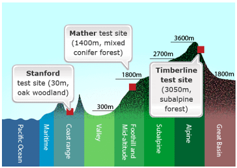 Locations for experimental studies examining contributions of G, E, and GxE. Adapted from Barbour at al., 1999
Conclusions
They concluded each species had differentiated into genetically distinct subspecies — which they called ecotypes — that are best suited to their specific environments. In the transplant gardens, no single ecotype performed best at all altitudes. For example, genotypes that produced the tallest plants at the mid-altitude garden site grew poorly at the low and high sites. Conversely, genotypes that grew the best at the low or high sites sometimes performed poorly at the mid-altitude site. Although within a species, all populations were found to be completely interfertile, ecotypes adapted to low or mid-altitude died when transplanted to the high altitude garden, while ecotypes from high elevations along the transect survived through the winter when locally grown in the test plots. GxE interaction was observed for height, among other characters.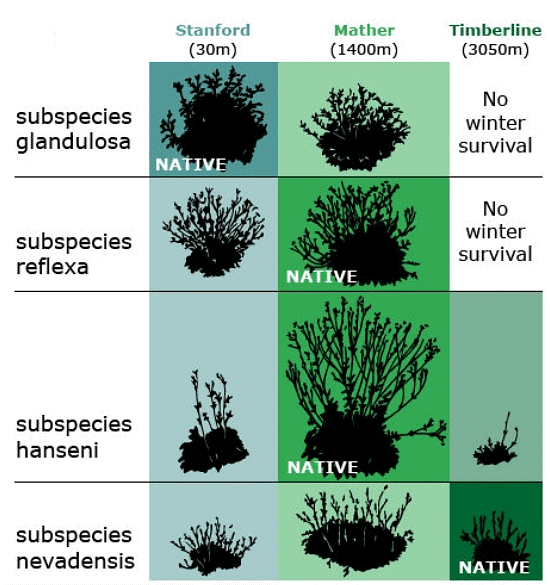 Response of plant ecotypes (Potentilla subspecies) to low, mid-, and high elevation transplant sites. Data from Clausen, Keck, and Hiesey, 1940, in Rauscher, 2005.
Significance Illustration
Figure 3 shows variation in phenotype between two cultivars of watermelon with regard to a quantitatively inherited trait (yield in this case) in response to variation in an environmental factor (soil salinity in this case) and illustrates the significance of genotype x environmental interaction.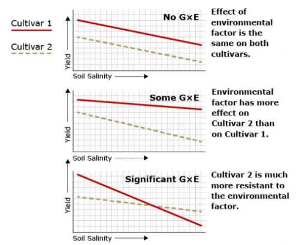 Hypothetical comparisons of genetic x environment interactions (GxE) in yield of two watermelon cultivars in response to increasing levels of soil salinity
Characteristics of Quantitative Traits
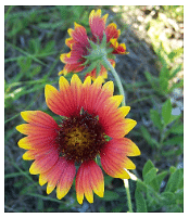 The diameter of Gaillardia pulchella flowers is a quantitative trait. Photo by DanielCD; CC-SA 3.0 via Wikimedia Commons
The inheritance of quantitative traits is governed by the interaction of multiple genes (polygenes) rather than single, distinct genes. These genes collectively influence the trait's expression, and their effects are also influenced by environmental factors. Unlike simple Mendelian traits where the impact of individual genes is clear, in quantitative traits, the contribution of each gene is not immediately apparent. However, it was later discovered in the early 1900s that the inheritance of the individual genes responsible for quantitative traits does adhere to the same Mendelian inheritance principles as single genes with distinct alleles.
Inheritance of Quantitative Traits
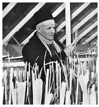 Herman Nilsson-Ehle. Photo licensed under Public Domain via Wikimedia Commons
- In 1909, Herman Nilsson-Ehle, a Swedish geneticist and wheat breeder, conducted seminal research on quantitatively inherited traits in wheat. His work led to the development of the "Multiple Factor" or multi-factorial theory of genetic transmission. One significant observation made by Nilsson-Ehle was that while a continuous range of kernel color variation (a quantitatively inherited trait influenced by environmental factors) was evident in the offspring generations, he was able to determine that the segregation of genes governing this trait followed Mendelian inheritance patterns.
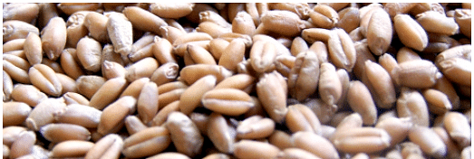 Wheat kernels. Photo by zandland; licensed under CC-SA 3.0
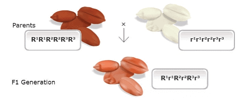
- Bread wheat, in particular, is a hexaploid and allopolyploid plant, meaning it has six sets of chromosomes and contains three slightly different ancestral genomes (referred to as A, B, and D) within its genome (AABBDD). Depending on the wheat cultivars that Nilsson-Ehle studied, each of these genomes had a single gene responsible for kernel color. Each of these loci had two alleles: a red allele (R) and a white allele (r). These alleles had slightly varying effects on kernel color and were designated using different superscripts, such as R1 or r3, to distinguish them.
- Nilsson-Ehle performed a cross between two wheat cultivars with differing kernel colors. One parent had dark red seeds (homozygous dominant genotype R1R1R2R2R3R3, based on the ancestral genomes), while the other parent had white kernels (homozygous recessive r1r1r2r2r3r3). He observed that the offspring of this cross (F1 generation), which had a heterozygous genotype (R1r1R2r2R3r3), exhibited an intermediate kernel color (light red). However, when he examined the second generation (F2 generation), he noticed that the individuals could be categorized into seven classes, ranging from dark red to white in kernel color. He explained this distribution by proposing that three pairs of genes were segregating independently, with each dominant allele contributing to the intensity of the red color in the kernels. In this way, he demonstrated that Mendelian genetics could account for the variation in this quantitatively inherited trait, even though the trait itself showed continuous variation.
Kernel color in F2 progenies from a wheat cross
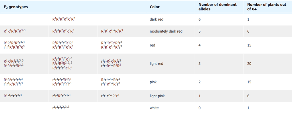
With three independent pairs of genes segregating, each with two alleles, as well as environmental effects acting on kernel color, the F2 progeny would contain 63 plants with varying shades of red kernels and one with white kernels. Linkage among the genes restricts independent assortment, so that the required size of the F2 population becomes larger.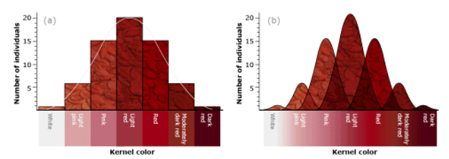 Range of wheat kernel color in an F2 generation. (a) Kernel color depicted by seven discrete classes modeled on segregation of three contributing genes, each exhibiting partial dominance. (b) Kernel color depicted by continuous variation in all seven color classes
Characteristics Indicative of Quantitative Inheritance
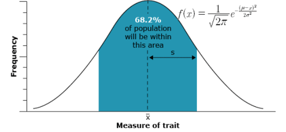 Based on a random sample from a genetically mixed population, the distribution of a quantitative trait’s expression approximates a normal or bell curve
- Phenotypic traits influenced by the simultaneous segregation of multiple genes display a spectrum of continuous variation, rather than distinct categories. Typically, the distribution of these quantitatively inherited traits within a population adheres to a normal distribution, often referred to as a Gaussian distribution or bell curve. These curves are characterized by two key parameters: the mean (represented by
 in a sample and μ in a population) and the variance or standard deviation (symbolized by s in a sample and σ in a population).
 - Quantitatively inherited traits can be categorized into three general types: continuous, meristic, and threshold traits. For instance, continuous traits, like the width of pineapple fruit, show a smooth range of values. Meristic characters, on the other hand, are traits counted in whole numbers only, such as the number of tillers in maize or branches on a rose bush. The third type of quantitative trait is known as a threshold character, where traits are typically categorized as either present or absent, without intermediate stages. An example of a threshold character is the presence or absence of Downy Mildew disease in soybeans.
- The environment plays a significant role in influencing the phenotype of this trait. In other words, how plants express this particular trait varies when they are grown in different environmental conditions.
- In contrast to traits controlled by individual, distinct genes with specific segregation ratios, this trait is influenced by multiple nonallelic genes. The patterns of recombination and segregation result from the combined impact of these polygenes on the trait. The more genetic loci that control the trait, the more complex its inheritance becomes.
- While genes may have different individual actions, their combined effect on the trait is cumulative. Various types of gene actions are involved, including additive effects, dominance, overdominance, and epistasis. These gene actions collectively shape the trait's phenotype. Appendix A delves into the effects of gene actions using concepts like genotypic and breeding values.

Summary of interactions among alleles (within or between loci) defining different types of gene action 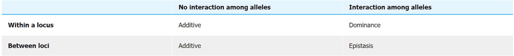
Transgressive segregation may occur. These individuals exhibit phenotypes outside the range of those expressed by the parents. Transgressive segregation occurs when progeny contain new combinations of multiple genes with more positive effects or more negative effects for the quantitative trait than found in either parent. One challenge is that strong environmental effects would make it difficult to assess the mean performance in parental plants vs. progeny in order to detect for the presence of any transgressive segregants.
Measurement of Continuous Variation
- When studying the inheritance of qualitative traits, the focus is typically on individual matings and their resulting offspring, and assessments are made through counts and ratios. In contrast, the study of quantitative traits involves populations of organisms with a wide range of potential mating scenarios, and the analysis of such traits relies on statistical methods. These statistical techniques serve as a valuable tool for describing and evaluating quantitatively inherited characteristics.
- Given the impracticality of examining an entire population, plant breeders opt to sample the population(s) they are interested in studying. It's crucial that this sample accurately represents the population, and to achieve this, the sample must meet two criteria:
- Adequate Size: The sample needs to be large enough to encompass the full spectrum of trait variability found within the population. The more diverse the trait within the population, the larger the required sample size to accurately represent it.
- Random Selection: To prevent any bias from skewing the results, the sample must be randomly selected, ensuring that each member of the population has an equal chance of being included.
- Therefore, the more extensive the variability within the population, the larger the sample size necessary to provide an accurate portrayal of that population. Throughout this and subsequent modules, it's generally assumed that we are referring to a representative sample rather than the entire population.
- Statistics used in this context can be broadly categorized as either descriptive or analytical, helping researchers not only describe the traits but also analyze their patterns and relationships within populations.
QTLs and Mapping
- The extent to which a particular trait is influenced by genetic or environmental factors can be estimated by studying the similarity in phenotype among relatives. In the past, quantitative genetics primarily relied on phenotypic data for such assessments. However, in recent times, molecular biology tools have become increasingly valuable for pinpointing the locations of quantitative trait loci (QTLs) within the genomes of plants and animals. These tools allow researchers to identify and map various genetic markers, making it possible to locate QTLs through linkage analysis.
- A common approach to mapping QTLs involves crossing two homozygous lines that possess different alleles at numerous genetic loci. The resulting F1 generation is then subjected to backcrossing and intercrossing, allowing genes to recombine through independent assortment and crossing over events. The subsequent generations, where offspring segregate, are carefully examined to identify correlations between the inheritance of marker alleles and the quantitative inheritance of phenotypes.
- It's important to note that QTL mapping is a complex process, and it will be explored in greater detail in future courses on Molecular Genetics and Biotechnology as well as Molecular Plant Breeding.
Multiple Genes and Gene Action
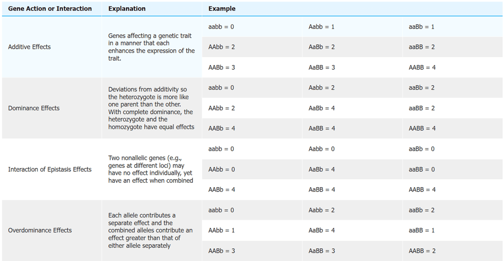
- The fundamental types of gene action for quantitative traits, including additive effects, full and partial dominance, and over-dominance, remain the same as those observed for qualitative traits. However, there are variations when it comes to quantitative traits due to the involvement of multiple genes, each with its unique gene action.
- In quantitative traits, the genes contributing to the phenotype may exhibit different individual gene actions, and their relative impacts on the trait's expression can vary. Some genes may exert a significant influence, while others may have only minor effects on the phenotype. Additionally, the genes controlling a quantitative trait may interact with each other, leading to complex patterns of gene action.
- The table below provides examples of gene action at two genetic loci. It's important to note that for quantitative traits, this concept is expanded to involve multiple loci, making the genetic basis of these traits more intricate and multifactorial.
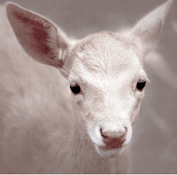 Albinism, such as that exhibited by this deer, is one common effect of pleiotropic mutation. Photo by Paulo Brandao; CC-SA 2.0
Heritability
Conceptual Basis for Understanding Heritability
Heritability estimates the relative contribution of genetic factors to the phenotypic variability observed in a population. What causes variance among plants and among lines or varieties? Phenotypic variation observed among plants or varieties is due to differences in
- their genetic makeup,
- environmental influences on each plant or genotype, and
- interaction of the genotype and environment.
The effectiveness with which selection can be expected to take advantage of variability depends on how much of that variability results from genetic differences. Why? Only genetic effects can be transmitted to progeny. Heritability estimates
- the degree of similarity between parent and progeny for a particular trait, and
- the effectiveness with which selection can be expected to take advantage of genetic variability.
Family Resemblance
As mentioned in the introduction of this lesson, central to the understanding of quantitatively inherited traits is the recognition of family resemblance. Two relatives, such as a parent and its offspring, two full or half-siblings, or identical twins, would be expected to be phenotypically more similar to each other than either is to a random individual from a population. Although close relatives may share not only genes (they may also share similar environments for traits that have a large genetic component), resemblance between relatives is expected to increase as closer pairs of relatives are examined because they share more and more genes in common. In this conceptual framework, heritability can be understood as a measure of the extent to which genetic differences in individuals contribute to differences in observed traits.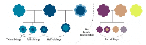 Individuals that are related genetically would be expected to be more phenotypically similar to each other than to other individuals from a population
Statistical Basis for Understanding Heritability
For plant breeders, heritability can also be understood in a statistical framework by defining it as the proportion of the phenotypic variance that is explained by genetic variance. Heritability indicates the proportion of the total phenotypic variance attributable to genetic effects, the portion of the variance that is transmittable to offspring. A general formula for calculating heritability is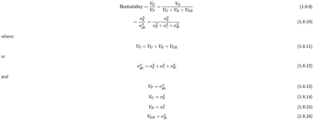
Uses of Heritability Estimates
- The concept of heritability is primarily used in the context of breeding decisions. It serves several purposes, including:
- Assessing the extent to which genetic factors can be passed from parents to offspring.
- Determining the most effective selection methods for improving a particular trait.
- Predicting the genetic progress that can be achieved through selective breeding.
- It's important to note that heritability estimates are specific to the population they are derived from and the environment in which that population was raised. However, some traits consistently exhibit either high or low heritability across different populations and environments. When dealing with traits that have high heritability, we can expect that the genotype of an organism will closely predict its phenotype across various environmental conditions. In other words, for traits with high heritability, the genetic makeup reliably determines the observable characteristics, unlike traits with low heritability, where the genetic influence is less predictable.
Characters
Heritability depends on the range of typical environments experienced by the population under study (if the environment is fairly uniform, then heritability can be high, but if the range of environmental differences is high, then heritability may be low. Even when heritability is high, environmental factors may influence a characteristic. Heritability does not indicate anything about the degree to which genes determine a trait; instead it indicates the degree to which genes determine variation in a trait.
Characters having low heritabilities are usually highly sensitive to the environment, presenting greater breeding challenges — low heritability traits often require larger populations and more test environments than do characters having high heritabilities for selection and improvement.
Table 4 Average heritability estimates (h2) of maize characters. Average estimates are derived from estimates reported in the literature. The magnitude of these estimates reflects both the complexity of the trait and the number of estimates reported in the literature.
Data from Hallauer and Miranda, 1988, p. 118.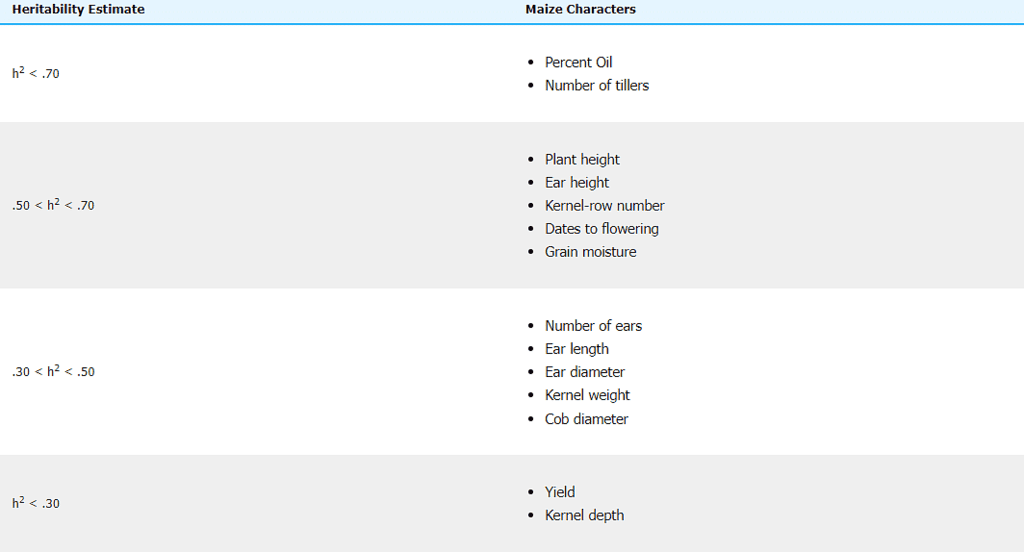
Broad-Sense Heritability
Types of Heritability
There are two types of heritability: broad-sense and narrow-sense heritability.
Broad-Sense Heritability
Broad sense heritability, H2, estimates heritability on the basis of all genetic effects.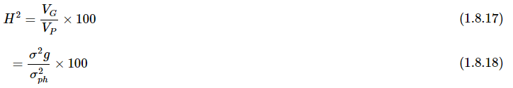
It expresses total genetic variance as a percentage, and does not separate the components of genetic variance such as additive, dominance, and epistatic effects.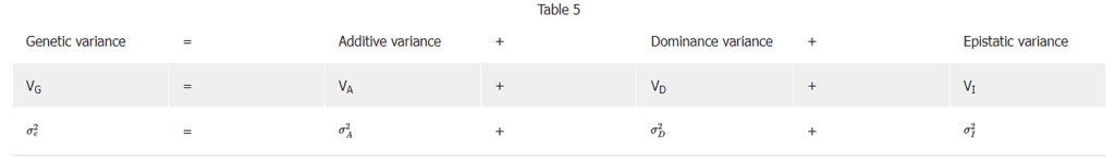
Generally, broad-sense heritability is a relatively poor predictor of potential genetic gain or breeding progress. Its usefulness depends on the particular population. Broad-sense heritability is
- more commonly used with asexually propagated crops than with sexually propagated agronomic crops
- applied to early generations of self-pollinated crops
Narrow-Sense Heritability
Narrow-sense heritability, h2, in contrast, expresses the percentage of genetic variance that is caused by additive gene action, VA.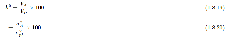
Narrow-sense heritability is always less than or equal to broad-sense heritability because narrow-sense heritability includes only additive effects, whereas broad-sense heritability is based on all genetic effects.
The usefulness of broad- vs. narrow-sense heritability depends on the generation and reproductive system of the particular population. In general, narrow-sense heritability is more useful than broad-sense heritability since only additive gene action can normally be transmitted to progeny. This is, because in systems with sexual reproduction, only gametes (alleles) but not genotypes are transmitted to offspring. In contrast, in case of asexual reproduction, genotypes are transmitted to offspring.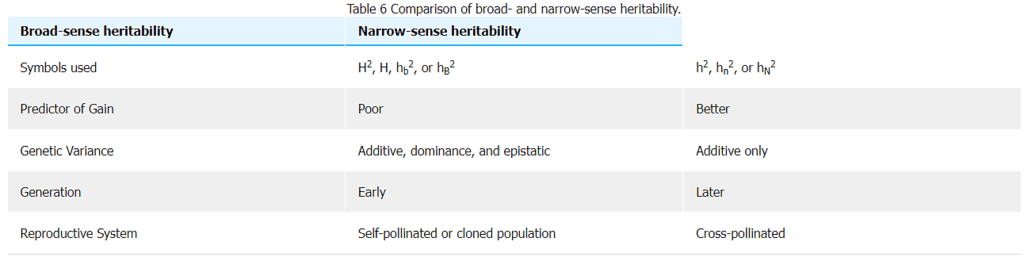
Estimating Heritability
There are two primary approaches to estimate heritability, which involve assessing the contributions of genetic (G), environmental (E), and genetic-environmental interactions (GxE) components. These methods can be used to calculate heritability and are typically derived from analyzing phenotypic variation within a population grown in different environments (across multiple locations and/or years).
Here are the two main approaches:
- Variance Component Approach: This approach involves dissecting the sources of variation in a trait through analysis of variance. By separating the total phenotypic variance into its genetic, environmental, and GxE components, one can estimate the proportion of phenotypic variation attributable to genetics, represented as heritability. This method often requires extensive data collection and statistical analysis to partition the sources of variation accurately.
- Parent-Offspring Resemblance Approach: In this approach, the focus is on comparing the resemblance between parents and their offspring with respect to the trait of interest. If there is a strong correlation between the phenotypes of parents and their offspring, it suggests a significant genetic contribution to the trait. This method is more straightforward in terms of data collection and can provide a quick estimate of heritability, particularly in situations where it may be challenging to conduct extensive environmental manipulations.
Both of these approaches aim to estimate heritability by considering the relative contributions of genetics, environment, and their interactions. The choice between these methods often depends on the availability of data and the specific characteristics of the population being studied.
Alternative Formula
An alternative formula for calculating the regression coefficient, b, is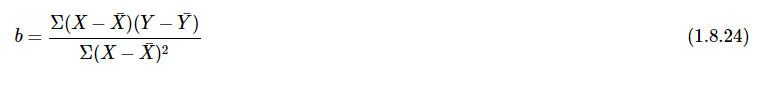
where:
b = regression coefficient
X = parent values
Y = progeny values
The performance of the progeny is a function of the genetic factors inherited from the parents. (Assume that “parent” means either a random plant or line from a population.) Thus, X, the parent value, is the independent variable, and Y, the progeny value, is the response or dependent variable.
Regression Coefficient
What does the regression coefficient, b, tell us?
If b = 1, then
gene action is completely additive,
negligible environmental effect,
and negligible experimental error.
The smaller the value of b, the less closely the progeny resemble their parent(s), indicating
greater environmental influence on the character,
greater dominance and/or epistatic effects, and/or
greater experimental error.
An analysis of variance will provide estimates of the relative influence of genetics, environment, and experimental error.
The type of heritability and the specific formula used to estimate it depends on the type of progeny evaluated.
Types of Progeny
The population’s reproductive mode and mating design determine the type of heritability and the formula used to calculate the estimate.
Selfed progeny
F2 plants are self-pollinated to obtain the F3. All the alleles in the F3 come from the F2 parent. Evaluate the character performance of the F3
Regress the performance of the F3 on the performance of their F2 parents.
The regression coefficient, b, is equal to H2, broad-sense heritability because its genetic variance includes dominance, additive, and epistatic effects.
Since it is difficult to obtain information about gene action (dominance, epistasis, additive) in self-pollinated populations, narrow-sense heritability is a poor predictor of genetic gain and rarely used in these populations. Inbreeding causes an upward bias in the heritability estimate.
Full-sib progeny
Two random F2 plants are mated. Half of the alleles in the F3 come from one parent and half from the other. Evaluate the character performance of the F3.
Determine the mid-parent value of the two parents. Mid-parent value, X = (x1 + x2) /2
Regress the progeny on the mid-parent value. The regression of progeny on the mid-parent value is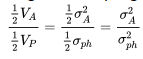
Since the progeny have both parents in common, only additive variance is included, so the regression coefficient, b, is equal to narrow-sense heritability.
h2 = b × 100 (1.8.25)
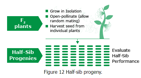
Half-sib progeny
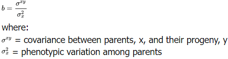
- Open-pollinate F2 plants. Seed will be harvested from each F2 individual separately. Progenies from the same F2 plant have the maternal parent (the respective F2 plant) in common, while the paternal parent is pollen from the whole F2 population. Thus all offspring from an F2 plant after open pollination are “half-sibs”.
- Regress the performance of the half-sib progenies on their parents.
- The covariance between parents and progeny includes additive variance and some forms of additive epistasis (usually negligible), but no dominance variance. Thus, narrow-sense heritability can be estimated. The regression coefficient, b, is equal to half the heritability value.
- Multiply the regression coefficient by 2 to obtain narrow-sense heritability.
h2 = 2b × 100 (1.8.26)
Heritability Influences
Heritability is not an intrinsic property of a trait or a population. As we’ve seen, it is influenced by:
- population — generation, reproductive system, and mating design
- environment — locations and/or years
- experimental design — experimental unit (plant, plot, etc.), replication, cultural practices, techniques for data gathering.
Heritability can be manipulated by increasing the number of replicates and number of environments sampled (in space and/or time). Genetic variance can be increased by using diverse parents and by increasing the selection intensity. Heritability is only an indicator to guide the breeder in making selections and is not a substitute for other considerations, such as breeding objectives and resource availability.
Genetic Advance from Selection
Evolution
Estimating Response to Selection
Evolution can be defined as genetic change in one or more inherited trait that takes place over time within a population or group of organisms. Plant breeders can use quantitative genetics to predict the rate and magnitude of genetic change. The amount and type of genetic variation affects how fast evolution can occur if selection is imposed on a phenotype.
The amount that a phenotype changes in one generation is called the selection response, R. The selection response is dependent on two factors—the narrow-sense heritability and the selection differential, S. The selection differential is a measure of the average superiority of individuals selected to be parents of the next generation.
R = h2S (1.8.27)
The above equation is often called the “breeder’s equation”. It shows the key point that response to selection increases when either the heritability of the trait or the strength of the selection increases.
Realized Heritability
In an experiment, the observed response to selection allows the calculation of an estimate of the narrow-sense heritability, often called the realized heritability. A low h2 (<0.01) occurs when offspring of the selected parents differ very little from the original population, even though there may be a large difference between the population as a whole and the selected parents. Conversely, a high h2 (> 0.6) occurs when progeny of the selected parents differ from the original population almost as much as the selected parents.
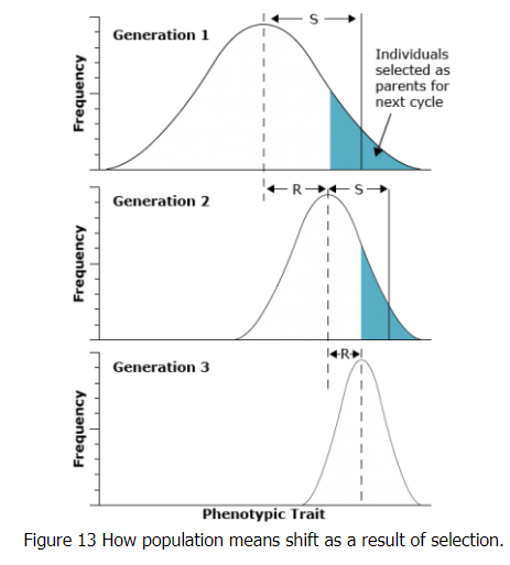
In the figure in the next screen, it can be seen that the selection differential (S) in each generation is the difference between the mean of the entire original population and the mean of group of individuals selected to form the next generation. In contrast, the response to selection (R) indicates the differences in population means across generations. The value of R is the difference between the mean of the offspring from the selected parents and the mean of the entire original population: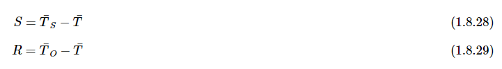
where:
- T = mean of the entire original population
- TS = mean of selected parents
- TO = mean of the offspring of the selected parents
Adaptive Value
The proportionate contribution of offspring of an individual to the next generation is referred to as fitness of the individual. Fitness is also sometimes called the adaptive value or selective value. Note in the figure that the non-selected members of the population do not contribute to the next generation and that selection over time reduced the variance of the population.
Types of Selection
Artificial selection refers to selective breeding of plants and animals by humans to produce populations with more desirable traits. Artificial selection is typically directional selection because it is applied to individuals at one extreme of the range of variation for the phenotype selected. This type of selection process is also called truncation selection because there is a threshold phenotypic value above which the individuals contribute and below which they do not. In contrast, under natural selection in non-managed populations, other types of selection may occur.
Three main types of selection are generally recognized. All three operate under natural selection in natural populations, whereas under artificial selection via selective breeding by humans only directional selection is common.
Directional Selection
Directional selection acts on one extreme of the range of variation for a particular characteristic.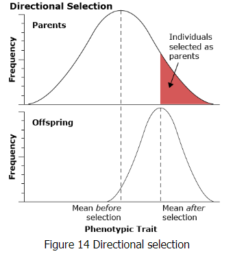
Stabilizing selection
Stabilizing selection works against the extremes in the distribution of the phenotype in the population. An example of this type of selection is human birth weight. Infants of intermediate weight have a much higher survival rate than infants who are either too large or too small.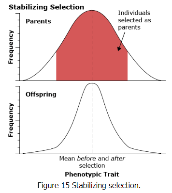
Disruptive selection
Disruptive selection favors the extremes and disfavors the middle of the range of the phenotype in the population.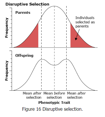
Genetic Advance from Selection
One of the most famous longest-term selection experiments is a study conducted by University of Illinois geneticists who have been selecting maize continuously for over 100 generations since 1896. They have been changing oil and protein content in separate experiments, selecting for either high or low content. In some cases after multiple generations, they have shifted selection from high to low or vice versa.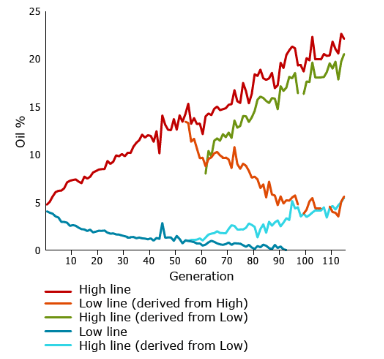
Figure 17 Responses to 100 generations for high and low oil concentration in maize kernels. Data from Department of Crop Science, University of Illinois at Urbana-Champaign, 2007.
Expected Gain From Selection
Because resources are limited, the breeder’s objective is to carry forward as few plants or lines as possible without omitting desirable ones. How does the breeder decide how many and which plants or lines within a population to carry forward to the next generation? The breeder can use heritability estimates to predict the probability that selecting a given percentage of the population or selection intensity, i, will result in progress. The expected progress or gain can be calculated using this formula:
where:
Gc = expected gain or predicted genetic advance from selection per cycle
k = selection intensity — a constant based on the percent selected and obtained from statistical tables (note that some people use hte i symbol instead of k for selection intensity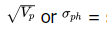 square root of phenotypic variance (equivalent to standard deviation)h2 = narrow – sense heritability in decimal form (narrow – sense is used for sexually reproduced populations whenever possible, and broad sense heritability, H2, is used for self – pollinating and asexually reproduce populations)Caution: The phenotypic values must exhibit a normal, or bell-curve, distribution for Gc to be valid
|
179 videos|140 docs
|
FAQs on Quantitative Genetics - Botany Optional for UPSC
| 1. What is heritability? |  |
| 2. What is the difference between heritable and environmental variation? | |
| 3. How is the inheritance of quantitative traits different from qualitative traits? | |
| 4. What is broad-sense heritability? | |
| 5. How is quantitative genetics relevant in the context of UPSC? | |

|
Nov 24, 2024 Last updated |

|
Explore Courses for UPSC exam
|
|
Quantitative Genetics | Botany Optional for UPSC
,Summary
,Objective type Questions
,past year papers
,MCQs
,Free
,shortcuts and tricks
,Quantitative Genetics | Botany Optional for UPSC
,practice quizzes
,study material
,video lectures
,Important questions
,Previous Year Questions with Solutions
,ppt
,Exam
,Sample Paper
,mock tests for examination
,Extra Questions
,Quantitative Genetics | Botany Optional for UPSC
,Viva Questions
,Semester Notes
;


Quantitative Genetics Free PDF Download
Importance of Quantitative Genetics
Quantitative Genetics Notes
Quantitative Genetics UPSC Questions
Study Quantitative Genetics on the App
|
© EduRev
|
Education Revolution
|


Follow Us
|