Linear Programming: Graphical Solution | Management Optional Notes for UPSC PDF Download
The graphical method is a convenient approach for solving simple linear programming (LP) problems. Simply follow these steps:
- Step 1: Plot the constraints on the graph paper to identify the feasible region.
- Step 2: Determine the coordinates of the corner points within the feasible region.
- Step 3: Calculate the values of the objective function at these corner points.
- Step 4: Select the corner point where the value of the objective function is maximum (or minimum, in the case of a minimization problem). This corner point will serve as the solution to the given LP problem.
Example: maximise z = 6x1 + 7x2
Subject to 2x1 + 3x2 ≤ 12
2x1 + X2 ≤ 8
(x1 x2) ≥ 0.

- The shaded region OAED is the set of points that are feasible under all the constraints it is called the feasible region. The task now is to find which combination of xi and \2 in OAED for which the value of z is maximised.
- The task is added by a theorem: If there exists an optimum solution to the problem, it will be found among the combinations of xj and X2 values represented by the vertices (or the extreme comers) of the feasible solution polygon.

- The value of z is maximum at E whose coordinates are (3, 2). Hence, the required solution is X1 = 3, x2 = 2 and the corresponding maximum value of z =32.
- The same process is followed for a minimisation process but only then we have to consider the minimum value of z.
Extra Variables
Before looking into further solution options of a LP, it will be useful to understand the nature of variables that enter into its formulation. For that purpose let us take a simple example: A textile firm produces two products I and II in its plant consisting of three departments dyeing, stitching and packaging. The machines in each department can be used for 8 hours a day. The production process can be described as follows:
- the product I is stitched first and then packaged. One ton of product I require 1/2 hour of stitching and y hour of packaging,
- product II is first dyed and than packaged. One ton of product II requires 1 hour of dying and 2/3 hours of packaging;
- products I and II are sold at prices Rs. 80 and Rs. 60 per ton respectively after the deduction of variable costs incurred;
- the gross profit per ton of products I and II is given as Rs. 40 and Rs. 30.
Our interest in the problem is to find out the output combination that would maximise the total profit of the firm.
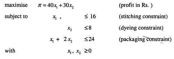
LP Formulation: Let x, andx, be the number of tons to be produced of products I and 11. The problem, therefore, is

We can rewrite the problems as:

Thus, there are altogether five variables. From these si( for I=l, 2, 3) are called slack variables. Note that the reformulated problem is equivalent to the original formulation except that the constraints are of the form
Ax = b
x = O
and we write the matrix equation as
When some component of x is of unrestricted sign, may be s3 ≥ 0 is omitted, then s, is calledfiee variable. You can eliminate a free variable by setting
s3 = u3, v3 where u3, v3 ≥ 0.
Two different standard forms of LP:
Observe that any LP can be converted to a problem in the form

This is because:
- Minimizing cTx is equivalent to maximizing -cTx,
- Inequalities in the constraints can be converted to equalities by adding by slack variables,
- Free variables can be eliminated as above.
Similarly, any LP can be converted into a problem in the from
since
The advantage of such a feature is that you can concentrate analysing any given forms of LP programming problem inter-ihangeably.
Assumptions of Linear Programming
- Divisibility: Decision variables in a linear programming model are allowed to have any values, including non-integer values that satisfy the constraints. Since each decision variable represents the level of some activity, it is being assumed that the activities can be run even at fractional levels.
- Proportionality: The contribution of each activity to the value of the objective function is proportional to the level of the activity Xj. Similarly, the contribution of each activity to the left-hand side of each constraint is proportional to the level of the activity Xj.
- Additivity: Every function in a linear, programming model is the sum of the individual contributions of the respective activities.
- Certainty: The value assigned to each parameter of a linear programming model is assumed to be a known constant.
FAQs on Linear Programming: Graphical Solution - Management Optional Notes for UPSC
| 1. What is linear programming? |  |
| 2. How is linear programming solved graphically? |  |
| 3. What is the significance of linear programming in the UPSC exam? |  |
| 4. Can linear programming be used in real-life scenarios? |  |
| 5. What are the limitations of linear programming? |  |


