Initial and boundary value problems

Definition of an Initial-Value Problem
An IVP is a differential equation together with a place for a solution to start. They are often written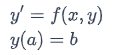
where
First Order Differential Equation Initial Value Problem
Let's start with the constant coefficient first order linear differential equation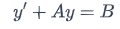
where A and B are real numbers with A ≠ 0. Remember that the general solution to this linear differential equation is 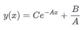 where C is a constant.
If you add the initial value  where x
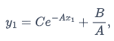 So,
So,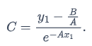 That means the solution to the IVP
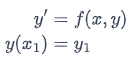
is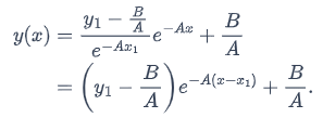
Initial value Problems and Separable Differential Equations
Remember that a differential equation is separable if you can write it in the form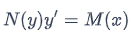
where N(y) and M(x) are functions. For more information and examples of this kind of equation see Separable Equations.
To make this into an IVP, all you need to do is pick an initial value. So for real numbers a and b, the IVP is 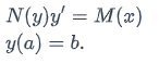
With separable equations, you often need to be careful with the interval of existence for solutions. In cases like that, the initial value tells you which of the intervals to choose as the interval of existence.
Let's take a look at an example.
Example: If possible, solve the IVP
Solution: First, you can rewrite the differential equation as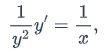 so it is a separable differential equation. Separating variables and integrating gives you
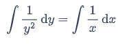
so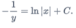 Now let's try and use the initial conditions. If you do, you will be using x = 0, and you can't take the natural log of zero. So in fact this IVP has no solution.
One more example, to see the kinds of things that can happen.
Example: Consider the IVP First show that the constant solution y(x) = 0 satisfies this IVP. Then see if there are any other solutions.
Solution: Certainly if you take the derivative of a constant function you get zero, and
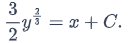
What about other solutions? This is a separable equation, so separating and integrating gives you
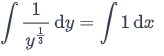
so
Using the initial value y
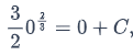
so C

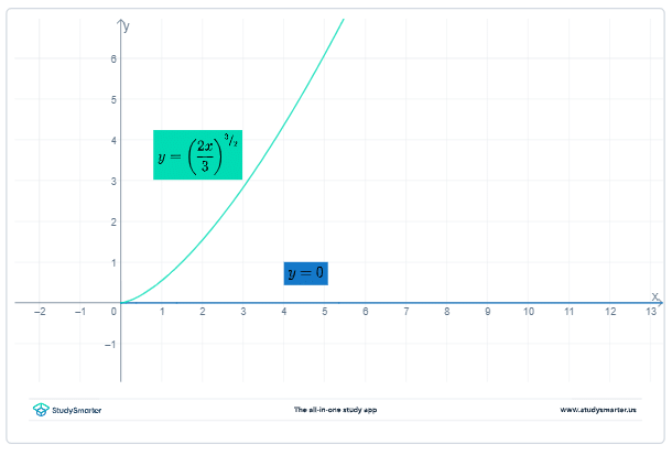
You can get the explicit solution by solving for y. If you do, you get
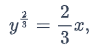
so
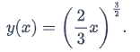
Notice that the maximal interval of existence is
More Solved Examples
Q1. Consider the problem y' = (1 - y2)10 cos y, y(0) = 0. Let J be the maximal interval of existence and K be the range of the solution of the above problem. Then which of the following statements are true?
Solution:
Concept -
(1) If f is bounded and continuously differentiable on R then maximum interval of existence is R.
We have y' = (1 - y2)10 cos y, y(0) = 0.
Now f(x,y) = (1 - y2)10 cos y
Clearly f is continuous and differentiable function.
Now |f| ≤ (1 - y2)10 ≤ M ∀ y ∈ R
Hence f is bounded as well
Therefore maximum interval of existence is R.
Now the function f = (1 - y2)10 cos y is even function as (1 - y2)10 is even and cos y is also even function.
⇒ y' = even
⇒ y = odd
Let assume y = x is odd function.
Now 1 = (1 - x2)10 cos x
Now according to the options, we take x = 1
then equation is not satisfied 1 ≠ 0
Hence the range of the solution (-1,1)
Q2. Consider the following initial value problem 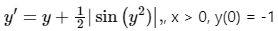 . Which of the following statements are true?
Solution:
We have 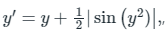 , x > 0, y(0) = -1
If a solution exist for the differential equation then Lipchitz condition is satisfied.
Now 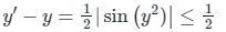
Now the solution of the differential equation is -
C.F. = C1ex PI =
PI =
Hence y = C1ex - 1/2
Now use the initial condition y(0) = -1 ⇒ C1 = -1/2
⇒ y = -1/2 ex - 1/2
⇒ y = -1/2 ex < 0
⇒ y is monotone decreasing.
Now 
but there does not exists an α ∈ (0, ∞)
Now as x → ∞ , y = -1/2 ex - 1/2 → - ∞ and y is decreasing as well.
So clearly it is not bounded below but it is bounded above.
Q3. Consider the initial value problem 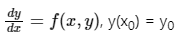 . where f is a twice continuously differentiable function on a rectangle containing the point (x0, y0). With the step-size h, let the first iterate of a second order scheme to approximate the solution of the above initial value problem be given by
y1 = y0 + Pk1 + Qk2,
where k1 = hf(x0, y0), k2 = hf(x0 + α0h, y0 + β0k1) and P, Q, α0, β0 ∈ ℝ.
Which of the following statements are correct?
Solution: the initial value problem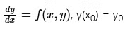
where f is a twice continuously differentiable function on a rectangle containing the point (x0, y0). With the step-size h, let the first iterate of a second order scheme to approximate the solution of the above initial value problem be given by
y1 = y0 + Pk1 + Qk2,
where k1 = hf(x0, y0), k2 = hf(x0 + α0h, y0 + β0k1) and P, Q, α0, β0 ∈ ℝ.
Compared with the Explicit Runge-Kutta method we get the relation,
P + Q = 1....(i)
Qα0 =1/2....(ii)
Qβ0 = 1/2....(iii)
Option (1):
If α0 = 2, then by (ii) Q = 1/4
Then by (iii), β0 = 2
Hence by (i) P = 3/4
Therefore we get
If α0 = 2, then β0 = 2,
Option (1) is true, (3) is false
Option (2):
If β0 = 2, then by (iii) Q = 1/6
Then by (ii), α0 = 3
Hence by (i) P = 5/6
Therefore we get
If β0 = 3, then α0 = 3,
Option (2) is true, (3) is false
FAQs on Initial and boundary value problems
| 1. What is an initial-value problem in the context of first-order differential equations? |  |
| 2. How are initial value problems related to separable differential equations? | |
| 3. How do initial and boundary value problems differ in the field of Mechanical Engineering? | |
| 4. Why are initial value problems important in the context of differential equations? | |
| 5. How can initial value problems be solved numerically in Mechanical Engineering applications? | |