Laplace transforms | Engineering Mathematics for Electrical Engineering - Electrical Engineering (EE) PDF Download

What is the Laplace Transform?
The Laplace Transform is a mathematical technique used to transform a function of a real variable t (often time) into a function of a complex variable s. This transformation simplifies the process of solving differential equations by converting them into algebraic equations.Piecewise Continuous Functions
A function f(t) is said to be piecewise continuous if it has a finite number of discontinuities and does not become infinite at any point. If f(t) is a piecewise continuous function, then its Laplace transform can be defined.
Definition of Laplace Transform
The Laplace transform of a function f(t) is represented as L{f(t)} or F(s). The transform is given by the integral formula: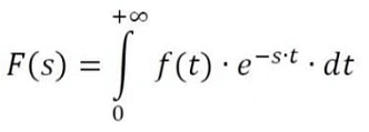 whenever the improper integral converges.
Standard notation: Where the notation is clear, we will use an uppercase letter to indicate the Laplace transform, e.g, L(f; s) = F(s).
The Laplace transform we defined is sometimes called the one-sided Laplace transform. There is a two-sided version where the integral goes from −∞ to ∞.
Properties of Laplace Transform
Some of the Laplace transformation properties are:If f1 (t) ⟷ F1 (s) and [note: ⟷ implies Laplace Transform]
f2 (t) ⟷ F2 (s), then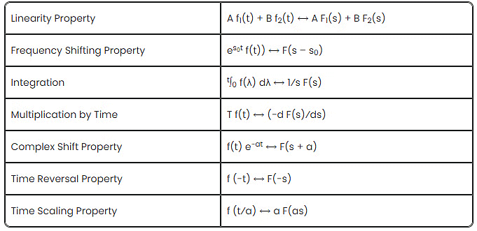
Laplace Transform Table
The following Laplace transform table helps to solve the differential equations for different functions: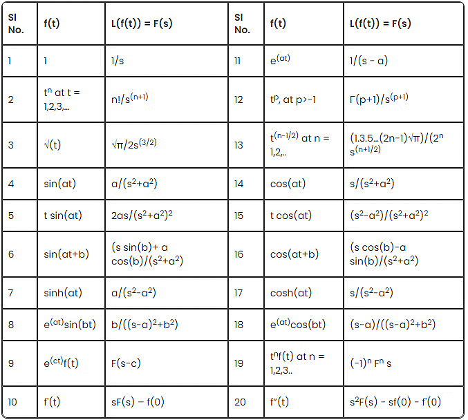
Laplace Transform of Differential Equation
The Laplace transform is a well established mathematical technique for solving a differential equation. Many mathematical problems are solved using transformations. The idea is to transform the problem into another problem that is easier to solve. On the other side, the inverse transform is helpful to calculate the solution to the given problem.For better understanding, let us solve a first-order differential equation with the help of Laplace transformation,
Consider y’- 2y = e3x and y(0) = -5. Find the value of L(y).
First step of the equation can be solved with the help of the linearity equation:
L(y’ – 2y] = L(e3x)
L(y’) – L(2y) = 1/(s-3)
(because L(eax) = 1/(s-a))
L(y’) – 2s(y) = 1/(s-3)
sL(y) – y(0) – 2L(y) = 1/(s-3)
(Using Linearity property of the Laplace transform)
L(y)(s-2) + 5 = 1/(s-3) (Use value of y(0) ie -5 (given))
L(y)(s-2) = 1/(s-3) – 5
L(y) = (-5s+16)/(s-2)(s-3) …..(1)
here (-5s+16)/(s-2)(s-3) can be written as -6/s-2 + 1/(s-3) using partial fraction method
(1) implies L(y) = -6/(s-2) + 1/(s-3)
L(y) = -6e2x + e3x
Step Functions
The step function is often called the Heaviside function, and it is defined as follows: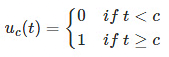 The step function can take the values of 0 or 1. It is like an on and off switch. The notations that represent the Heaviside functions are uc(t) or u(t-c) or H(t-c)
Bilateral Laplace Transform
The Laplace transform can also be defined as bilateral Laplace transform. This is also known as two-sided Laplace transform, which can be performed by extending the limits of integration to be the entire real axis. Hence, the common unilateral Laplace transform becomes a special case of Bilateral Laplace transform, where the function definition is transformed is multiplied by the Heaviside step function.The bilateral Laplace transform is defined as: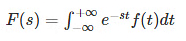
The other way to represent the bilateral Laplace transform is B{F}, instead of F.
Inverse Laplace Transform
In the inverse Laplace transform, we are provided with the transform F(s) and asked to find what function we have initially. The inverse transform of the function F(s) is given by:f(t) = L-1{F(s)}
For example, for the two Laplace transform, say F(s) and G(s), the inverse Laplace transform is defined by:
L-1{aF(s)+bG(s)}= a L-1{F(s)}+bL-1 {G(s)}
Where a and b are constants.
In this case, we can take the inverse transform for the individual transforms, and add their constant values in their respective places, and perform the operation to get the result.
Laplace Transform in Probability Theory
In pure and applied probability theory, the Laplace transform is defined as the expected value. If X is the random variable with probability density function, say f, then the Laplace transform of f is given as the expectation of:L{f}(S) = E[e-sX], which is referred to as the Laplace transform of random variable X itself.
Applications of Laplace Transform
- It is used to convert complex differential equations to a simpler form having polynomials.
- It is used to convert derivatives into multiple domain variables and then convert the polynomials back to the differential equation using Inverse Laplace transform.
- It is used in the telecommunication field to send signals to both the sides of the medium. For example, when the signals are sent through the phone then they are first converted into a time-varying wave and then superimposed on the medium.
- It is also used for many engineering tasks such as Electrical Circuit Analysis, Digital Signal Processing, System Modelling, etc.
Laplace Equation
Laplace’s equation, a second-order partial differential equation, is widely helpful in physics and maths. The Laplace equation states that the sum of the second-order partial derivatives of f, the unknown function, equals zero for the Cartesian coordinates. The two-dimensional Laplace equation for the function f can be written as: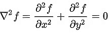
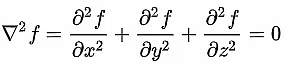
The Laplace equation for three-dimensional coordinates can be represented as:
Solved Numericals
Q1. If f(t) = eat, its Laplace Transform (for s > a) is given by
Solution: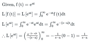
∴ Laplace transform is 
Q2. Consider the differential equation 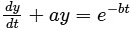 with the initial condition y(0) = 0. Then the Laplace transform Y(s) of the solution y(t) is
Solution: 
Integrating factor = 
Solution of y is,
Given that, y(0) = 0
Now, the solution becomes,
Apply Laplace transform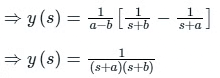
Q3. The Laplace transform of the differential equation y" + ay' + by = f(t). Assume that y(0) = 5, y'(0) = 10, Y(s) and F(s) are the Laplace transforms of y(t) and f(t) respectively
Solution: A second-order differential equation is represented as:
y" + ay' + by = f(t)
The Laplace transform of the above equation with the initial condition is:

Calculation
Given, y(0) = 5, y'(0) = 10
Q4. The inverse Laplace transform of 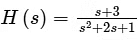 for t ≥ 0 is
Solution: Some pairs of Laplace transforms are given below.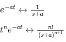
Given: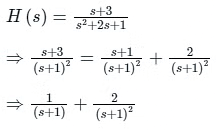
By applying inverse Laplace transform
⇒ H(t) = e-t + 2t e-t
Q5. If the Laplace transform of function f(t) is given by  , then f(0) is
Solution: Laplace Transforms: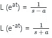
Given: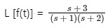
The above equation through partial fractions can be written as: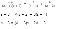
Comparing co-efficients on both sides, we get
A + B = 1 and 2A + B = 3
We get, A = 2, B = -1
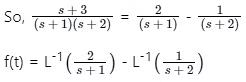
f(t) = 2e-t - e-2tSo,
f(0) = 2e-0 - e-0 = 2 - 1 = 1
∴ f(0) = 1
|
44 videos|109 docs|58 tests
|


MCQs
,past year papers
,Sample Paper
,Laplace transforms | Engineering Mathematics for Electrical Engineering - Electrical Engineering (EE)
,practice quizzes
,ppt
,Objective type Questions
,Extra Questions
,Semester Notes
,video lectures
,Viva Questions
,Summary
,Laplace transforms | Engineering Mathematics for Electrical Engineering - Electrical Engineering (EE)
,Important questions
,Free
,Exam
,Laplace transforms | Engineering Mathematics for Electrical Engineering - Electrical Engineering (EE)
,mock tests for examination
,Previous Year Questions with Solutions
,shortcuts and tricks
,study material
;


Laplace transforms Free PDF Download
Importance of Laplace transforms
Laplace transforms Notes
Laplace transforms Electrical Engineering (EE) Questions
Study Laplace transforms on the App
|
© EduRev
|
Education Revolution
|


|


